3. From the UPPE to the generalised nonlinear Schrödinger equation#
The generalised nonlinear Schrödinger equation (GNLSE) is probably the equation you know best. It has a dispersion operator, a nonlinear coefficient \(\gamma\), a self-steepening term and a Raman convolution, and it is the workhorse of fibre supercontinuum modelling (Dudley, Genty and Coen 2006). This chapter derives it from the UPPE of Chapter 2. The point is not that the derivation is new. The point is to see precisely which choices turn one equation into the other, because each choice is also a limitation: one transverse mode with a frozen profile, an effective area, a fitted dispersion relation and a carrier-frequency coefficient.
You will see where \(\gamma=n_2\omega_0/(cA_{\rm eff})\) comes from and what the effective area does and does not preserve. You will see why the shock term is \(\omega/\omega_0\) and why a frequency-dependent area is not one model but several. You will also see how the Raman fraction is accounted for, which quantity the equation conserves, and the characteristic lengths that organise soliton dynamics. The chapter ends with when the GNLSE is enough and when it is not.
3.1 One mode, one area#
Take the modal UPPE of §2.5 and keep a single mode with transverse profile \(F(x,y)\). If the nonlinear polarisation is computed from the field \(a(t)F(x,y)\) and projected back onto \(F\), the transverse integrals reduce to one number. For the Kerr effect, the projection of \(|E|^2E\) onto the mode involves \(\int|F|^4\,\mathrm dA\), normalised by \((\int|F|^2\,\mathrm dA)^2\). Its inverse is the effective area
(Dudley, Genty and Coen 2006, Eq. 1; mode averaging). Kolesik, Wright and Moloney (2004) make the point cleanly in their modal UPPE for silica nanowires. The GNLSE follows from a single replacement: the mode profile \(\mathcal M(\omega,r)\), which depends on frequency, is frozen at its shape at one reference frequency. Everything else in their Appendix follows from that.
Two things are worth holding on to.
The effective area preserves exactly one thing: the cubic self-coupling overlap. It does not preserve the local intensity. For the \(\mathrm{HE}_{11}\) mode of a capillary, whose profile is \(J_0(2.405\,r/a)\), the effective area is about \(1.50\,a^2\), and the on-axis intensity is \(1.768\) times \(P/A_{\rm eff}\) (spatial decompositions). For a Kerr response that does not matter, because the area was defined to make the Kerr overlap right. For a response that is a steep function of intensity, such as tunnelling ionisation, it matters a great deal. The rate at the peak of the mode and the rate at the effective-area intensity can differ by orders of magnitude (Chapter 10).
A frozen profile cannot change. It cannot self-focus, cannot couple to another mode and cannot narrow with frequency, so a mode-averaged calculation cannot predict any of those things. Chapter 5 removes the restriction.
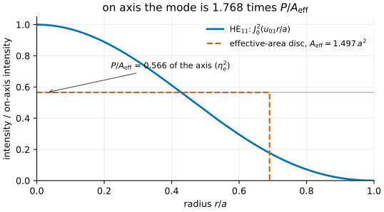
The \(\mathrm{HE}_{11}\) intensity across the core and the uniform disc with the same effective
area. The disc reproduces the cubic overlap exactly, but its intensity, \(P/A_{\rm eff}\), is
only 57% of the mode’s on-axis intensity. Computed in closed form by
docs/primer/figures/primer_figures.py.#
solprop distinguishes a mode-averaged calculation, with one amplitude and one area, from
a resolved single-mode calculation, with one amplitude but the nonlinear response
evaluated at quadrature nodes across the mode and projected back. prop_gnlse is the
former. prop_capillary(modes=1) is the latter. The difference is invisible for Kerr and
essential for ionisation (mode averaging).
3.2 From the polarisation to \(\gamma\)#
Follow the coefficient through once, for a continuous wave so that no transform is involved. Let the modal amplitude \(A\) be normalised so that \(|A|^2\) is the power in watts. The field it represents, for the effective-area model, is
so that \(\tfrac12\varepsilon_0c|E_a|^2=|A|^2/A_{\rm eff}\) is a vacuum-admittance intensity (watts and volts per metre). The Kerr polarisation of the envelope is \(P=\tfrac34\varepsilon_0\chi^{(3)}|E_a|^2E_a\) (§1.6). Apply the UPPE prefactor \(i\omega/(2\varepsilon_0c)\) with the index set to one (more on that below), and convert back from field to amplitude with the same factor:
At \(\omega=\omega_0\) this is \(i\gamma|A|^2A\) with
the textbook nonlinear coefficient (Dudley, Genty and Coen 2006, below Eq. 2). The same chain, in the internal convention, is the identity that solprop’s test suite asserts on both grids (it comes out as the textbook equation).
The usual relation in a medium of linear index \(n_0\) is \(n_2=3\chi^{(3)}/(4\varepsilon_0cn_0^2)\).
The GNLSE route takes \(n_0=1\) in that relation and in the prefactor, consistently. A GNLSE
dispersion relation is a fitted \(\beta(\omega)\), routinely written with \(\beta_0=0\), and
not a physical effective index, so \(c\beta/\omega\) cannot stand in for the index. solprop
records the choice on the problem as prefactor_index
(the coefficient mapping). In
reverse, prop_gnlse turns your \(\gamma\) into a susceptibility with
where \(f_R\) is the Raman fraction of §3.5. Other bookkeepings are equally consistent if applied throughout. Lægsgaard (2007, Eq. 19) keeps the factor \(\omega/(c\,n_{\rm eff}(\omega))\) and so defines \(n_2\) with one power of \(n_0\), not two, and says so. When you take an \(n_2\) from a paper, check which definition it uses.
The same coefficient appears in field-level forward equations written without an envelope: Brabec and Krausz (2000, Sec. V) in the optics sign, and Guo et al. (2013, Eq. 1) in the FFT sign, where it is exactly solprop’s internal prefactor. Copy such equations with care. The sign of the nonlinear term in Brabec and Krausz’s Eq. 26 does not match their own transform convention, although their envelope equation, Eq. 29, is consistent.
3.3 The linear part: Taylor series or the exact \(\beta(\omega)\)#
In the optics convention the envelope’s linear propagation is \(\partial_z\tilde A=i[\beta(\omega)-\beta_0-\beta_1(\omega-\omega_0)]\tilde A-\tfrac12\alpha\tilde A\). Expanding \(\beta\) about \(\omega_0\) and using \((\omega-\omega_0)\to i\partial_T\) gives the familiar time-domain operator
with \(T=t-\beta_1z\) the retarded time. Dudley, Genty and Coen (2006, Sec. IV.A) already recommend the alternative: “given \(\beta(\omega)\) the dispersion operator can be applied directly and in an approximation-free manner in the frequency domain”. A spectral code pays nothing for doing so, and the Taylor series has a finite radius of convergence set by the material’s resonances (§1.3). Adding more orders does not help (Amiranashvili, Vladimirov and Bandelow 2010; Amiranashvili, Bandelow and Mielke 2012). For a guide, its own resonances and cut-offs limit the radius further.
solprop’s prop_gnlse takes a fibre as a SpecifiedMode:
a Taylor series about the reference frequency, a cubic-spline table, or a callable. It uses
it exactly in the frequency domain, with an analytic derivative for the frame. It refuses
to extrapolate a table outside the data it was built from (“the classic way to get a
plausible, wrong answer”), and offers no constructor that expands a Taylor series about
zero frequency
(the fibre is a mode). On the capillary
and waveguide routes there is no Taylor series at all. The mode supplies its complex
\(n_{\rm eff}(\omega)\) at every frequency of the grid (Chapter 4).
3.4 Self-steepening and the frequency-dependent coefficient#
Chapter 2 showed that the \(\omega\) in the numerator of the UPPE prefactor is the optical shock. On an envelope, \(\omega/\omega_0=1+(\omega-\omega_0)/\omega_0\to1+\tfrac{i}{\omega_0}\partial_T\), and the nonlinear term becomes
the form of Brabec and Krausz (1997, Eq. 6), of Dudley, Genty and Coen (2006, Eq. 2) with
\(\tau_{\rm shock}=1/\omega_0\), and of Kolesik, Wright and Moloney (2004, Eq. A.26).
solprop does not carry the time-domain derivative. With shock=True it multiplies the
transformed polarisation by \(\omega\) exactly, which is the non-perturbative form. With
shock=False it freezes the numerator at the carrier
(the shock term). The term is not a small
correction. For the deep-ultraviolet dispersive wave of an argon-filled kagomé fibre, Joly
et al. (2011) computed 11.3% conversion with it and 3.2% without, because the
dispersive-wave emission depends exponentially on the spectral amplitude at the pulse’s
blue edge, which the shock enhances.
Three different frequency dependences are easily confused here, and solprop keeps them apart:
The UPPE frequency factor. This is the \(\omega\) of the prefactor, a property of the output frequency of the polarisation, switched by
shock. In the envelope limit it is self-steepening.Modal dispersion of the nonlinearity. The effective area and the overlap change with frequency because the mode changes shape. This is a geometric property of the guide.
Material dispersion of \(\chi^{(3)}\). The susceptibility depends on all four frequencies of each four-wave-mixing quartet. A GNLSE \(\gamma\) is one fitted constant, so it has none of this. Chapter 8 discusses the gas models that do.
The second of these has a tangled literature, and it is worth knowing that “the GNLSE with a frequency-dependent area” is not one model. Dudley, Genty and Coen (2006, Eq. 3) correct the shock time to \(\tau_{\rm shock}=\tau_0-[\mathrm d\ln n_{\rm eff}/\mathrm d\omega]_{\omega_0}-[\mathrm d\ln A_{\rm eff}/\mathrm d\omega]_{\omega_0}\), which is the first-order expansion of a coefficient proportional to \(\omega/(n_{\rm eff}(\omega)A_{\rm eff}(\omega))\) evaluated at the output frequency. Lægsgaard (2007) shows that putting \(A_{\rm eff}(\omega)\) at the output frequency “is obviously not well founded”. The correct single-mode equation involves an overlap of four mode profiles at four frequencies (his Eqs. 16–17). The variant that conserves photon number, accurate to first order in \(\omega-\omega_0\), divides every field by \(A_{\rm eff}^{1/4}(\omega)\) (his Eqs. 33–34). Lægsgaard credits that form, in a slightly different shape, to Mamyshev and Chernikov (1990). In those rescaled variables the area term of the shock coefficient is half of Dudley’s. That is not a contradiction: the two equations use different variables.
solprop’s scalar GNLSE route holds the area at its value at the reference frequency, so its shock time is exactly \(1/\omega_0\). At 835 nm that is 0.443 fs. Dudley, Genty and Coen’s canonical photonic-crystal-fibre simulation used 0.56 fs, from their Eq. 3. A solprop run of “Dudley’s case” is therefore not quite the same model in the shock term. When the frequency dependence of the mode matters, the right tool is the general modal route, which carries the mode shapes at every frequency and does the four-frequency projection properly (Chapter 5).
3.5 The Raman fraction#
Silica and molecular gases have a delayed, nuclear contribution to the nonlinearity as well as the instantaneous electronic one. The GNLSE writes the total response as \(R(t)=(1-f_R)\delta(t)+f_Rh_R(t)\), with \(h_R\) normalised to unit integral, so that
(Dudley, Genty and Coen 2006, Eq. 2). Here \(\gamma\) is the total nonlinearity, and \(f_R\) says how it is shared. For silica, \(f_R=0.18\) is traditional. Chapter 9 explains where the other values come from, including 0.2188 for the default silica response in solprop.
The bookkeeping between a field-level Raman response and the envelope’s \(f_R\) hides a factor of \(\tfrac23\). The Raman polarisation is driven by \(E^2\). Averaged over a cycle, \(E^2\to\tfrac12|E_a|^2\), whereas the Kerr cubic gives \(\tfrac34|E_a|^2E_a\). A Raman term whose susceptibility integrates to \(X\) therefore acts like a Kerr term of \(\tfrac23X\), and on this route, whose kernel is an effective one at density one and unit index, the share \(f_R\) of the total \(\chi^{(3)}\) corresponds to
(the Raman fraction is not silently taken). Bache (2016, Eqs. 21–26) gives the same accounting and argues that the generalised envelope equation of Genty, Kinsler, Kibler and Dudley (2007) omits this factor, so that using \(f_R=0.18\) there underestimates the Raman effect by \(\tfrac23\). solprop does the accounting Bache’s way.
The other question is what “no Raman” means. prop_gnlse defaults to raman=False, and
then gives the whole of \(\gamma\) to the Kerr term. A pair of runs that switches only
raman then keeps the soliton order and the self-phase modulation, and differs only in the
delay of the response. If instead you want the delayed part removed and the instantaneous
part left as it was, pass the fraction explicitly. A given raman_fraction is always held
back from the Kerr term. The difference is not small: holding back silica’s fraction without
a Raman response turns an “\(N=6\)” soliton into \(N=5.30\).
3.6 What the equation conserves#
With the shock term on and no loss, the GNLSE does not conserve energy. It conserves the photon number, \(\sum_k|\tilde A(\omega_k)|^2/\omega_k\). The Raman response moves photons to lower frequency, and each one then carries less energy than it brought. Chernikov and Mamyshev (1991, Eqs. 2–6) give the cleanest statement: any change of energy or mean frequency “can be associated only with the imaginary part of the Raman susceptibility”. Mamyshev and Chernikov (1990, Eq. 10) and Lægsgaard (2007, Eq. 35) show which form of the frequency-dependent coefficient keeps that invariant.
solprop’s guide records the measurement. Over a hundredth of a soliton period with
\(f_R=0.18\), the photon number is conserved exactly and the energy falls by
\(7.2\times10^{-6}\). With shock=False the equation conserves energy instead, which is the
wrong invariant for a delayed response. With Raman off, both hold to round-off
(which invariant the equation has).
Dudley, Genty and Coen (2006, Sec. IV.B) recommend monitoring the photon number as a
numerical check. Chapter 13 explains why such a check is necessary but far from
sufficient.
3.7 Characteristic lengths and the soliton#
The GNLSE has two natural length scales, one for dispersion and one for the nonlinearity:
for a pulse of peak power \(P_0\) and duration parameter \(T_0\) (\(T_0=T_{\rm FWHM}/1.763\) for a sech pulse). In anomalous dispersion, \(\beta_2<0\), an \(N=1\) sech pulse is the fundamental soliton. Higher-order solitons breathe with period \(z_{\rm sol}=\tfrac\pi2L_D\). A perturbed \(N\)-soliton breaks up near the fission length \(L_{\rm fiss}\sim L_D/N\) (Dudley, Genty and Coen 2006, Sec. V.B.1). The constituent fundamental solitons have peak powers \(P_0(2N-2j+1)^2/N^2\) and durations \(T_0/(2N-2j+1)\) (Dudley, Genty and Coen 2006, Sec. V.B.1). solprop’s design tools compute these numbers from a guide, a gas and a pulse. They also stress that \(N\) is a continuous measure of nonlinearity, not the number of solitons that emerge. For pulses long enough that \(N\gtrsim10\), noise-seeded modulational instability tends to overtake fission (Genty, Coen and Dudley 2007).
The numbers are worth carrying in your head, because they show why gas-filled fibres and solid-core fibres behave so differently. Dudley, Genty and Coen’s photonic-crystal fibre has \(\gamma=0.11\) W⁻¹m⁻¹ and \(\beta_2=-11.8\) ps²/km at 835 nm. For a 50 fs pulse \(L_D\) is about 7 cm, and 10 kW gives \(N\approx8.5\). Travers et al. (2011) give \(\gamma\approx2\times10^{-6}\) W⁻¹m⁻¹ for a 30 µm hollow core filled with 10 bar of argon, smaller by a factor of about \(5\times10^4\). The dispersion of such a guide is also smaller by orders of magnitude, so that the same soliton orders are reached at microjoule to millijoule energies. Travers et al. (2011, Eq. 4) show that, for Kerr-driven dynamics of a given pump, the zero-dispersion wavelength and \(N\) organise the regimes: combinations of core size, gas, pressure and energy that give the same pair give similar dynamics. Identical evolution would also need matching higher-order dispersion, shock parameter \(1/\omega_0T_0\), pulse shape, loss and length. “It makes no sense to compare \(\lambda_0\) or N on their own.”
A soliton has a nonlinear wavenumber of half its peak nonlinear phase rate, \(\gamma P/2\). It is robust because that wavenumber lies where no linear wave can exist. Higher-order dispersion opens a resonance, and the soliton then sheds a resonant dispersive wave at the frequency where the linear wavenumber matches its own:
(Akhmediev and Karlsson 1995, Eqs. 2 and 5a; Travers et al. 2011, Eq. 8). Dudley, Genty and Coen (2006, Sec. V.B.2) write the same condition with \((1-f_R)\gamma P_s\) and no factor \(\tfrac12\). For a sech fundamental soliton the \(\tfrac12\) is right, and solprop’s phase-matching tool uses it. Mixing of solitons with dispersive waves adds further four-wave-mixing resonances (Skryabin and Yulin 2005, Eq. 11). These dynamics are the subject of the lessons and the examples. The point here is only that every one of these estimates comes from the GNLSE, while the full calculation uses the UPPE with the exact dispersion.
3.8 When the GNLSE is enough#
The GNLSE is the right model when one mode carries the pulse, its profile hardly changes over the spectrum, the response is Kerr and Raman, and the spectrum stays narrow enough for an envelope. That covers a great deal of solid-core fibre optics and many gas-filled fibre problems. solprop runs it on an envelope grid, with exactly the same stepper, output and backends as everything else.
It stops being enough in any of these cases.
When ionisation matters. The rate depends steeply on the local field, so the effective-area intensity is the wrong input. Use a resolved single mode or a mode set, and converge the radial rule (Chapters 5 and 10).
When energy moves between modes. A capillary pumped at high energy, a taper or a graded-index fibre all transfer energy between modes. Use a mode set (Chapter 5).
When the mode changes shape across the spectrum. Supercontinua spanning octaves in small-core fibres, and nanowires, need the general modal route. Its vector \(\gamma\) for a 250 nm silica strand is 25% above the scalar one (solid-core fibres).
When the carrier matters. Third-harmonic generation and sub-cycle dynamics need a field grid (Chapter 11).
When the material \(\chi^{(3)}\) is dispersive. A single \(\gamma\) cannot represent a frequency-dependent Kerr coefficient (Chapter 8).
All of these routes solve the UPPE of Chapter 2. The GNLSE is not a different physics, only the UPPE with the transverse dimension collapsed onto one frozen profile and an index of one.
What to remember
The effective area \(A_{\rm eff}=(\int|F|^2)^2/\int|F|^4\) preserves only the cubic self-coupling overlap. On axis, \(\mathrm{HE}_{11}\) has 1.768 times \(P/A_{\rm eff}\).
\(\gamma=n_2\omega_0/(cA_{\rm eff})\) comes from the UPPE prefactor, the \(\tfrac34\) of the envelope cubic and the field–amplitude conversion. solprop’s GNLSE route takes the index as one, consistently, and records it.
Apply the exact \(\beta(\omega)\) in the frequency domain where you can. Taylor series have a radius of convergence, and solprop never extrapolates a tabulated dispersion.
Self-steepening is \(\omega/\omega_0\). A frequency-dependent area is a separate effect and not a single well-defined model; solprop’s GNLSE holds the area fixed, so \(\tau_{\rm shock}=1/\omega_0\) exactly.
\(\int h\,\mathrm dt=\tfrac32f_R\chi^{(3)}_{\rm total}\), with \(h\) the field-level Raman susceptibility (\(h_R\) has unit integral). With
raman=Falseand no given fraction, all of \(\gamma\) is Kerr.With the shock on, the invariant is photon number, not energy.
\(L_D=T_0^2/|\beta_2|\), \(L_{\rm NL}=1/\gamma P_0\), \(N^2=L_D/L_{\rm NL}\), \(L_{\rm fiss}\sim L_D/N\). The phase-matching condition carries \(\tfrac12\gamma P\).
The precise statements are in generalised nonlinear Schrödinger propagation, mode averaging and design tools. Chapter 4 opens the transverse dimension again and asks what a waveguide mode is.