Solid-core fibres: the general modal route

This chapter is for solid-core fibres whose modes matter as they are — vector, frequency-dependent, with their longitudinal field: step-index fibres with their exact vector modes, graded-index multimode fibres, declared polarisation bases and fibres that taper. (A single-mode fibre described by \(\gamma\) and \(\beta(\omega)\) alone is faster on prop_gnlse; see the GNLSE.)

A solid-core fibre is propagated on its own modes: a provider solves the fibre’s electric and magnetic fields — all three components of each — at quadrature nodes across the cross-section, at every frequency the run needs, and the run evaluates the material’s nonlinear response at those nodes and projects it back onto the modes, which this route calls channels. Resolving the vector field matters in a strongly guiding core: on a 250 nm silica strand, the longitudinal field and the \(|\mathbf E\cdot\mathbf E|^2\) term make the vector nonlinear coefficient 25 % larger than the scalar \(n_2\omega/(cA_{\rm eff})\). The model and its derivation are described in general modal propagation and the chapters after it (a tapered guide in moving modal bases); the measured checks against independent references are in the qualification record. This chapter is how to use the route.

What the route carries: on a 250 nm silica strand in air, the transverse field of \(\mathrm{HE}_{11}\) at the provider’s nodes (arrows), and beneath it the longitudinal field \(E_z\), comparable with the transverse one. All three components enter the nonlinear response at every node. Figures of every transverse decomposition are on spatial decompositions.

The route is three objects, built in order:

1. the regions — the materials of the cross-section, each with its own responses;

2. the guide — a provider, solved on its own node rule at frequency knots spanning the run’s whole active band (ModalGuide);

3. the run — prop_waveguide((), length, provider=guide, ...) or Simulation.from_waveguide(..., provider=guide).

A step-index fibre, with its vector modes

StepIndexMode is an exact vector mode of a circular step-index fibre: kind is the family ("HE", "EH", "TE", "TM"), n the azimuthal and m the radial order, parity which member of a degenerate pair. Here the two parities of \(\mathrm{HE}_{11}\) and the \(\mathrm{TE}_{01}\)/\(\mathrm{TM}_{01}\) pair of a 6 µm core, the Kerr response declared on the core and nothing on the cladding — which is how a region is said to be linear.

The exact mode of a step-index guide is not truncated: along x the field is radial and jumps by the permittivity ratio at the core boundary; along y it is tangential and continuous.

import numpy as np

from solprop.driver import prop_waveguide
from solprop.grid import FieldGrid
from solprop.modes import (
    IndexMaterial,
    MaterialKerr,
    MaterialRegion,
    ModalGuide,
    StepIndexMode,
)

RADIUS = 6e-6
core, cladding = IndexMaterial(1.45), IndexMaterial(1.44)
modes = [
    StepIndexMode(
        RADIUS,
        core=1.45,
        cladding=1.44,
        profile_wavelength=835e-9,
        kind=kind,
        n=n,
        m=1,
        parity=parity,
    )
    for kind, n, parity in (
        ("HE", 1, "even"),
        ("HE", 1, "odd"),
        ("TE", 0, "even"),
        ("TM", 0, "even"),
    )
]
regions = (
    MaterialRegion("core", 0.0, RADIUS, core, (MaterialKerr(n2=2.6e-20, at=835e-9),)),
    MaterialRegion("cladding", RADIUS, None, cladding),
)
provider = ModalGuide.from_step_index(
    modes, core=core, cladding=cladding, regions=regions
).field_provider

The guide must be solved over the run’s whole active band, which runs from half the grid’s lowest declared frequency to its highest — so a grid declared over 790–890 nm needs a guide from 1.8 µm down. Every channel must still be bound at that long end (a \(\mathrm{TE}_{01}\) of a 4 µm core is not, and is refused by name), and the node rule must resolve the fields there, where they reach furthest into the cladding. The knots are the frequencies the provider is solved at; between them the fields are interpolated, and the route gates the interpolated basis’s departure from orthonormal (gram_atol, 1e-4) where the launched spectrum is, and warns (GeneralModalBasisWarning) where it is not but light could go. More knots is the fix for both. The knots are always yours: no provider or constructor chooses them. For a dispersive core spread them geometrically in frequency (np.geomspace), which crowds them towards the infrared where the index curves: with a Sellmeier silica core over an active band from 3.6 µm to 450 nm, linearly spaced knots fail the propagation-constant check (PROVIDER_BETA_RTOL) at the infrared end even at 81, where 97 geometrically spaced ones pass.

length = 1e-3
grid = FieldGrid.from_limits(length, 835e-9, (790e-9, 890e-9), 200e-15)
active = grid.omega[grid.active_mask]
low, high = 0.99 * float(active[0]), 1.01 * float(active[-1])
guide = ModalGuide.from_provider(
    provider,
    np.linspace(low, high, 25),
    nodes=provider.node_rule(low, n_r=24),
    degenerate_blocks=((0, 1),),  # the two parities of HE11
)
print(guide)

degenerate_blocks names the channels the provider declares degenerate, so that the tracking between knots may rotate freely inside the pair instead of matching an order its equal eigenvalues cannot resolve. The printed block lists the channels by label — HE1,1:even, HE1,1:odd, TE0,1, TM0,1 — and those labels are how a launch names a channel:

output = prop_waveguide(
    (),
    length,
    provider=guide,
    grid=grid,
    channel="HE1,1:even",
    lambda0=835e-9,
    fwhm=40e-15,
    energy=1e-10,
    n_save=3,
    dz_max=length / 10,
    dz_init=length / 10,
    progress="none",
)
print(output["stats/physical_energy"])

provider= takes the guide, not the provider. Every gas keyword (gas, pressure, kerr, raman, n_r, …) is refused beside it by name, because the guide owns its materials, responses and transverse rule. The launched amplitude is the pulse’s own, unchanged: every channel is normalised to unit Poynting flux, so a channel amplitude already is a true-power amplitude in √W.

What a region may declare. MaterialKerr by chi3= or by n2=; an n2 needs the wavelength it was measured at, at=, whenever the region’s index moves the converted \(\chi^{(3)}\) by more than one per cent across the band (a dispersive silica core does; the refusal says so). Beside it, SilicaTensorResponse adds the delayed Lin–Agrawal tensor Raman response of fused silica, sharing the region’s one \(\chi^{(3)}\):

from solprop.nonlinear.raman import SilicaTensorResponse

raman_core = MaterialRegion(
    "core",
    0.0,
    RADIUS,
    core,
    (MaterialKerr(n2=2.6e-20, at=835e-9), SilicaTensorResponse()),
)
print(raman_core)

Which cubic. The kerr_form= keyword of prop_waveguide chooses how the Kerr response is evaluated. kerr_form="real", the default, is the real-field cubic, which radiates the third harmonic and needs the grid’s room for it (FieldGrid’s default oversampling has it); kerr_form="analytic" carries the fundamental band alone — what an envelope route models, and the right choice for a like-for-like comparison with prop_gnlse. The two agree on the fundamental to rounding.

What it costs. A general modal step synthesises the field at every node and frequency and projects it back, so it costs roughly the node count times the channel count times the frequency count, about a hundred times a capillary step of the same grid. The dense maps and the stored E/H reference are held for the whole run (16 × nodes × components × channels × n_omega bytes each): the backends chapter says how that is estimated and budgeted before anything is allocated.

A graded-index multimode fibre

GradedIndexProvider solves a radial core law — here the parabola PowerLawPermittivity — by finite elements matched to the exact Bessel exterior. family is "TE" or "TM" for the vector sectors of azimuthal order zero, or "LP" for the weak-guidance scalar sector (permittivity contrast up to 0.02, no longitudinal field) with azimuthal_order; count is the number of consecutive radial channels; elements and extent are the discretisation, explicit because they are numerical choices to refine. The core’s responses are declared on the provider itself, core_responses=; its exterior is always linear.

The provider’s node rule splits at every finite element of the core and at the matching radius; beyond it the field is an exact Bessel continuation, not nodes.

from solprop.modes import GradedIndexProvider, PowerLawPermittivity

grin = GradedIndexProvider(
    permittivity=PowerLawPermittivity(IndexMaterial(1.45), 0.005),
    exterior=IndexMaterial(1.45 * np.sqrt(1.0 - 2.0 * 0.005)),
    radius=25e-6,
    family="LP",
    count=2,
    elements=32,
    extent=2.0,
    core_responses=(MaterialKerr(n2=2.6e-20, at=1.03e-6),),
)
grin_grid = FieldGrid.from_limits(1e-3, 1.03e-6, (1.0e-6, 1.06e-6), 100e-15)
grin_active = grin_grid.omega[grin_grid.active_mask]
grin_low = 0.99 * float(grin_active[0])
grin_guide = ModalGuide.from_provider(
    grin,
    np.linspace(grin_low, 1.01 * float(grin_active[-1]), 13),
    nodes=grin.node_rule(grin_low, n_r=2),
)
print(grin_guide)

A centred beam excites only the radially symmetric channels, so an LP sector of azimuthal order zero is the natural basis for an on-axis launch. Its fields have no angular dependence, so its node rule takes two angular nodes by default, which are exact (a TE/TM sector takes nine, a higher LP order more). The number of channels is bounded by what is still bound at the long end of the active band; a channel too near cutoff there is refused by name, with the fraction of its power beyond the matching radius. A larger core or contrast, or a grid that reaches less far into the infrared, admits more.

A launch declared as an incident beam. incident= takes a SpatialPulse, whose energy is met over the whole beam at the entrance, in the core medium, and coupling= the model it is coupled under (coupling simulations). The beam’s coordinates in every channel are recovered through the Poynting pairing; the channels launch what they capture, and the rest is lost at the entrance rather than restored. The coupling’s report – incident and launched energy per frequency and its admission budget – is recorded in the run’s configuration (CouplingReport).

from solprop.coupling import CouplingModel
from solprop.pulses import GaussianPulse, SpatialPulse

beam = SpatialPulse(  # an x-polarised Gaussian, 12 um waist, at its waist
    GaussianPulse(wavelength=1.03e-6, fwhm=50e-15, energy=1e-9), 12e-6
)
grin_run = prop_waveguide(
    (),
    1e-3,
    provider=grin_guide,
    grid=grin_grid,
    incident=beam,
    coupling=CouplingModel("vector_paraxial", model_error=0.2),
    lambda0=1.03e-6,
    n_save=3,
    dz_max=1e-4,
    dz_init=1e-4,
    progress="none",
)
launch = grin_run.metadata.configuration["launch"]
print(f"launched {launch.efficiency:.3f} of the beam within {launch.budget:.3f}")

The graded-index core’s contrast, 0.005, is below the budget’s eighth, as the vector model requires (general modal propagation). The recovered amplitudes are launched unscaled, so the run’s physical_energy at the entrance is the launched energy, not energy=.

The graded-index worked example runs a 100 µm core at full power over ten centimetres: self-imaging, geometric parametric instability and the exchange of energy between the channels.

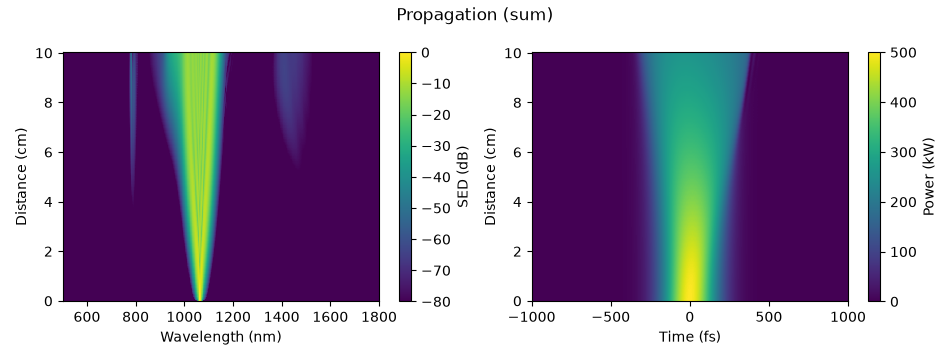
From the worked example: the spectrum (left) and the power (right) along the fibre, summed over the four channels. Self-phase modulation broadens the pump, and the geometric parametric instability of the self-imaging beam grows sidebands near 800 nm and 1.45 µm.

Declared bases: circular polarisation and split pairs

A guide’s channels come in the basis its provider solved them in — for a degenerate pair, the real parity pair. Any unitary combination is as good a basis, and one of them is physically special: the circular pair, for which \(\mathbf E\cdot\mathbf E\) vanishes, the \((\mathbf E\cdot\mathbf E)\mathbf E^*\) term of the Kerr cubic drops out and the self-phase coefficient falls to two thirds of its value for linear polarisation. circular_pair() declares it; from_provider takes it as basis=:

from solprop.modes.guide import circular_pair, provider_channels

circular = ModalGuide.from_provider(
    provider,
    np.linspace(low, high, 25),
    nodes=provider.node_rule(low, n_r=24),
    degenerate_blocks=((0, 1),),
    basis=circular_pair(provider_channels(provider), (0, 1)),
)
print([label.display_label for label in circular.mode_collection.channel_labels])

With this basis the channels are HE1,1:left and HE1,1:right (the block’s first member must be the even one; the other order is refused). The run’s metric becomes the dense Hermitian one of the declared basis, the noise is drawn in the provider’s basis and carried through the transform, and the declaration is part of the file’s resume key. The conditions on the basis and the dense metric are in declaring a circular basis.

A block that is only nearly degenerate — split by the vector correction, by stress, by a bend — can be declared too, with ChannelBasis: the rotated channels then genuinely beat, and the run carries the block as a coupled flow. What a rotated channel reports, what is withheld and what is refused beside it are in a declared basis of a block that is only nearly degenerate; A declared basis of a split pair: two bases, one answer runs one against the provider’s own basis.

A solid guide that moves along z

A tapered step-index fibre, a graded-index multimode taper or a photonic lantern propagates with its own mode fields at every position: give ModalGuide.from_provider a provider whose geometry moves along z, and the guide is re-solved along the path at the Chebyshev degree its own held-out check demands, the synthesis and projection maps move with the modes, and the solid-mode connection \(\langle\psi_m|\partial_z\psi_n\rangle\) converts the launch between the channels in the frozen-section flow. The model, its validation and its limits are in moving modal bases. It runs on all three backends, numpy_ref, numba_cpu and native (CPU and GPU builds). A strong taper couples strongly: the run’s advisory step warns when the steps are too long, and sections= shortens the frozen sections. Beside a moving guide a noise model, a lockstep batch, a CF4 flow and a fixed schedule that straddles a kink of the path are refused. The tapered graded-index worked example runs eight tapers from abrupt to adiabatic against a first-order coupled-mode estimate and Love’s criterion, rebuilds the fields at the entrance and the waist, and puts a self-phase-modulating pulse through a taper beside the scalar area model.

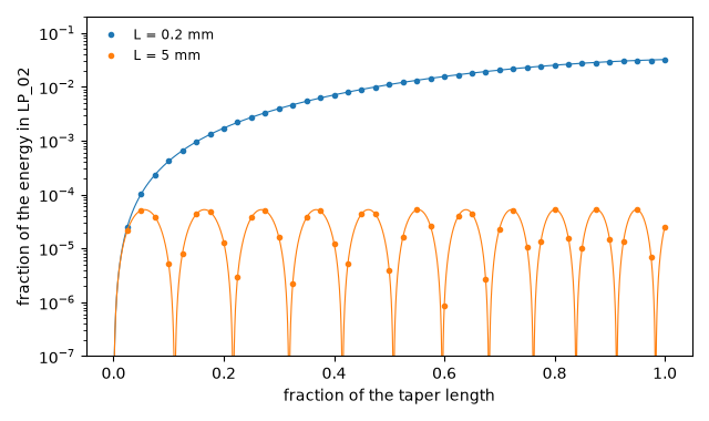
From the worked example: the energy converted from \(\mathrm{LP}_{01}\) into \(\mathrm{LP}_{02}\) along an abrupt taper (0.2 mm) and a slow one (5 mm). The runs (dots) lie on the first-order coupled-mode estimate (lines).

What the route refuses, and why

Every refusal names itself, at the entry point and again in the translation layer and the backend; the complete list, with the reason for each, is declared, refused, recorded. The ones a user meets first:

• a guide that does not span the active band, or a channel not bound at its long end;

• a node rule that truncates or under-resolves the fields (the sampled basis is further from orthonormal than gram_atol) — refine the rule (n_r) or widen it;

• knots too sparse for the provider’s own propagation constants between them — add knots (for a dispersive material, geometric spacing in frequency helps: the knots crowd towards the infrared, where the index curves);

• an n2 without at= on a dispersive core, and the real cubic on a grid with no room for its harmonic;

• the per-channel power statistics (energy, peak_power, …), replaced by physical_energy and analytic_flux (reading the output);

• on a moving guide, a noise model, a lockstep batch, a CF4 flow or a fixed schedule that straddles a kink (above).

The incident-beam launch into a fibre and its coupling budget were proposed and carried out by SEP 31.