The linear operator#

Linear propagation sets the dispersion, attenuation and reference frame in which the pulse evolves. A moving frame removes the common carrier or group delay so that the numerical window follows the pulse; relative delays and dispersion remain physical effects. The RDW lesson and crossing-beam lesson show their temporal and spatial consequences.

This chapter defines the operator and its signs. Varying operators explains the interpolation and cumulative integral for pressure gradients and tapers. Exact integration of a represented diagonal operator does not make an approximate material law or interpolation exact.

In the frequency domain each mode obeys

\[ \partial_z a_m(\omega,z) = [D_m(\omega,z)-\tfrac12\partial_z\ln w_m(\omega,z)]a_m(\omega,z)+N_m[a](\omega,z), \]

where \(a\) is the internal vacuum-normalised modal amplitude, \(N_m\) the nonlinear term (nonlinear responses) and \(w=\operatorname{Re}n_{\rm eff}\), or the explicit constant index a run declares in its place. The saved amplitude is the true-power \(b=\sqrt w a\) (power, energy and intensity); the logarithmic term keeps its energy right where \(w\) varies along z, and vanishes for a constant fill and on the GNLSE mapping. The dispersion operator

\[ D_m(\omega, z) = -\mathrm{i}\bigl(\beta_m(\omega, z) - \beta_0(z) - \beta_1(z)(\omega - \omega_0)\bigr) - \tfrac{1}{2}\alpha_m(\omega, z) - \tfrac{1}{2}\alpha_\text{abs}(\omega) \]

carries the dispersion and the loss of the mode in a co-moving frame, plus the spectral absorbing collar expressed as a rate. The \(\beta_0\) term is removed only on an envelope grid without a third-harmonic term; a field grid keeps it and measures the \(\beta_1\) term from zero frequency, for the reasons given under which terms the frame removes. Signs, units and the Fourier convention are fixed in the conventions; this page uses the internal FFT convention throughout.

For independent modal channels, D is diagonal in frequency and channel. Its values at different positions commute, giving the diagonal linear flow

\[ \tilde E(\omega, z_2) = \exp\bigl(\Phi(\omega, z_2) - \Phi(\omega, z_1)\bigr)\,\tilde E(\omega, z_1), \qquad \Phi(\omega, z) = \int_0^z D(\omega, z')\,\mathrm{d}z' - \tfrac12\ln\frac{w(\omega,z)}{w(\omega,0)} , \]

for the stated \(\Phi\), at any step length. Evaluating the z-dependent operator at one point per step instead — a right-endpoint rule, say — is globally first order in the step and invisible to the embedded error estimate. solprop represents \(\Phi\) with a controlled table or parameter expansion. The diagonal homogeneous flow is exponential, while source variation, coupled terms and absorbers still impose accuracy or stability requirements; the evidence is in the stepper notes, section 4, and the choice is among the design decisions.

Where channels exchange power linearly — the capillary’s coherent wall, the taper coupling of a multimode capillary taper, or a split block of the general modal route — the linear part is not diagonal in the channel axis. Such a run keeps a diagonal operator common to every channel — the carrier, or one reference channel’s dispersion — and carries each channel’s departure from it, and the coupling, as a separate coupled linear flow. This page describes the diagonal part, which every run has.

Assembly and the frame#

D is assembled by solprop.linear.dispersion_operator() from three things: a mode, a grid, and a solprop.linear.Frame.

From the effective index#

Everything the mode supplies enters through its complex effective index. With \(k = \omega/c\),

\[ \beta(\omega, z) = \frac{\omega}{c}\,\mathrm{Re}\,n_\text{eff}(\omega, z), \qquad \alpha(\omega, z) = \frac{2\omega}{c}\,\mathrm{Im}\,n_\text{eff}(\omega, z), \]

so that \(\mathrm{Im}\,n_\text{eff} > 0\) is loss and the field amplitude decays as \(\mathrm{e}^{-\alpha z/2}\) while the power decays as \(\mathrm{e}^{-\alpha z}\). These are the definitions of the conventions §2.

The frame quantities come from the same index, differentiated analytically (solprop.linear.frame_quantities()):

\[ \beta_0 = \frac{\omega_\text{ref}}{c}\,\mathrm{Re}\,n_\text{eff}(\omega_\text{ref}), \qquad \beta_1 = \frac{1}{c}\left(\mathrm{Re}\,n_\text{eff} + \omega_\text{ref}\,\mathrm{Re}\frac{\mathrm{d}n_\text{eff}}{\mathrm{d}\omega} \right)_{\omega_\text{ref}} . \]

Only the real part appears, so the loss never moves the frame. Mode.dneff_domega is required to be analytic because a differenced \(\beta_1\) has a roughness floor near \(5\times10^{-8}\) that would cap the whole table at \(10^{-8}\); recomputing it every stage from a finite-difference stencil would also cost several index evaluations per stage.

Which terms the frame removes#

The frame subtracts a constant \(\beta_0\) and a linear \(\beta_1(\omega - \omega_\text{ref})\). The linear term is a change of time origin: it keeps the pulse in the window on a gradient fibre, which a fixed frame does not. The constant term is a change of carrier phase. Which of them applies depends on the grid, because the two grids store different objects:

grid	operator
field	\(-\mathrm{i}\,(\beta - \beta_1\omega) - \alpha/2\)
envelope, no third harmonic	\(-\mathrm{i}\,(\beta - \beta_0 - \beta_1(\omega - \omega_\text{ref})) - \alpha/2\)
envelope, with third harmonic	\(-\mathrm{i}\,(\beta - \beta_1\omega) - \alpha/2\)

The two grids that keep \(\beta_0\) propagate a source that follows the carrier at \(\kappa = \beta(\omega_0) - \beta_1\omega_0\) per metre, which the default Adams integrator has to resolve; the carrier frame removes that rotation inside each step.

A field grid stores the real field. Multiplying its half-spectrum by a frequency-independent phase is not a global phase at all: it rotates the carrier-envelope phase of the field, which drives ionisation and the third harmonic. So \(\beta_0\) is not removed there, and the frame term is measured from zero frequency, because a pure delay is a phase linear in \(\omega\) through the origin.

An envelope grid has already had the carrier taken out, so removing \(\beta_0\) as well simply stops the envelope spinning at \(\beta_0\) per metre. The exception is a third-harmonic term: its \(\mathrm{e}^{2\mathrm{i}\omega_0 t}\) factor is tied to the true carrier phase (see the nonlinear responses), and removing \(\beta_0\) would shift the harmonic relative to the fundamental. Such a frame keeps the carrier phase whole, so its delay is measured from zero frequency, exactly as on a field grid. Measured from \(\omega_\text{ref}\), the term \(\beta_1(\omega - \omega_\text{ref})\) would still remove a constant \(-\beta_1\omega_\text{ref}\): the envelope would turn at \(\beta_1\omega_\text{ref}\) per metre and \(A^3\) at three times that, while the harmonic’s carrier factor is fixed in time, so the third harmonic would be driven with a spurious mismatch of \(2\beta_1\omega_\text{ref}\), about \(1.2\times10^{7}\ \mathrm{rad/m}\) in a gas at 1 µm, against a true \(\beta(3\omega_0) - 3\beta(\omega_0)\) of order \(10^{3}\)–\(10^{4}\ \mathrm{rad/m}\) in a gas-filled capillary. A frame that keeps \(\beta_0\) on an envelope grid therefore always measures its delay from zero (solprop.linear.frame_origin()). the conventions §2 writes the envelope form for both grids, which is the right formula in the case it is usually read for. solprop.linear.Frame.comoving() picks the rule from the grid.

Either way, a single reference frequency is used for \(\beta_0\), \(\beta_1\) and the \((\omega - \omega_\text{ref})\) offset; two different references would be consistent only up to a constant phase.

One frame for a mode set#

\(\beta_m\) carries a mode index in the operator at the top of this page; \(\beta_0\) and \(\beta_1\) do not, and that is not shorthand. A multimode problem uses one frame for the whole set, taken from the first mode, at every position along \(z\).

The reason is that the \(\beta_1\omega\) term is a change of the time variable. Removing each mode’s own \(\beta_1\) would put every mode in its own time origin, and the set would no longer be simultaneous: mode \(p\) would drift against mode 1 by \((\beta_{1,p} - \beta_{1,1})z\). That drift is the group-delay walk-off, and it is physics — for \(\mathrm{HE}_{11}\) against \(\mathrm{HE}_{12}\) of a 125 µm capillary at 800 nm it is 43 fs per metre, tens of pulse widths over a metre of fibre. The nonlinear term multiplies the modes at the same time sample (the nonlinear responses), so a set written in per-mode frames has its walk-off silently transformed away and its intermodal coupling evaluated on fields that were never simultaneous. On a four-mode resonant-dispersive-wave (RDW) capillary run, per-mode frames under-populate the higher modes by two to four orders of magnitude.

solprop.linear.Frame recomputes \(\beta_0\) and \(\beta_1\) from the mode it is handed, which is what makes the frame co-moving on a gradient fibre; the mode set is known one layer up, so solprop.translate.linop.build_phi() freezes the frame on the first mode at each position before evaluating the columns. Those are also the quantities it tabulates beside \(\Phi\), so the record and the operator say the same thing. A mode-averaged problem has one mode and is unaffected either way.

Where the operator is evaluated#

The mode is evaluated on the grid’s active band, \(\omega_\text{min}/2 < \omega < 1.1\,\omega_\text{max}\), and D is zero outside it. That is not laziness: an effective index is \(c\beta/\omega\) and has no value at zero frequency, which a field grid contains, and the state outside the active band is removed each step by the hard band mask (absorbing boundaries).

The spectral absorber, in contrast, is added over the whole axis. With the collar expressed as a rate rather than a per-step window, out-of-band bins have to carry it: with a zero operator there they would propagate loss-free. dispersion_operator takes the rate as an array, so the collar geometry stays in boundaries.

The loss policy#

An effective index can produce an arbitrarily large \(\alpha\): a capillary bin below cutoff, a table asked for a frequency it does not cover. Two things then go wrong. \(\mathrm{e}^{-\alpha z/2}\) underflows, and the adaptive Chebyshev builder spends intervals resolving a bin whose field is zero. Fixed empirical clamps on \(\alpha\) or on the index would answer both, but a constant chosen without reference to the fibre can change an answer.

solprop answers with a limit derived from the fibre. solprop.linear.LossPolicy caps \(\alpha\) at

\[ \alpha_\text{max} = \frac{2 \times 708}{L}, \]

\(708\) being the largest exponent whose \(\mathrm{e}^{-x}\) is still a normal double. At that loss the transmitted amplitude has already underflowed over the whole fibre, so no clamp placed there can change an answer. There is no lower limit: gain is representable and is never clamped to zero. A non-finite index raises rather than passing through. The clamp is applied to D itself, before \(\Phi\) is integrated — clamping the accumulated exponent instead would make the answer depend on the step.

The operator of a dispersion-specified fibre#

import matplotlib.pyplot as plt
import numpy as np

from solprop.constants import C
from solprop.grid import EnvelopeGrid
from solprop.linear import Frame, dispersion_operator
from solprop.nonlinear.gnlse import SpecifiedMode

grid = EnvelopeGrid.from_limits(0.1, 1030e-9, (700e-9, 2e-6), 2e-12)
omega0 = grid.omega0
mode = SpecifiedMode.from_taylor(
    [1.45 * omega0 / C, 1.47 / C, 2.0e-26, -1.0e-41], omega_ref=omega0, aeff=8e-11
)

active = grid.active_mask
omega = grid.omega[active]
order = np.argsort(omega)
wavelength = 2e9 * np.pi * C / omega[order]

fig, ax = plt.subplots(figsize=(6.4, 3.4), layout="constrained")
labels = {"comoving": "co-moving", "delay": r"$\beta_1$ only", "lab": "lab frame"}
frames = {
    "comoving": Frame.comoving(grid),
    "delay": Frame(omega0, subtract_beta0=False),
    "lab": Frame(omega0, subtract_beta0=False, beta0=0.0, beta1=0.0),
}
for name, frame in frames.items():
    phase = -np.imag(dispersion_operator(mode, grid, frame))[active][order]
    ax.plot(wavelength, phase, lw=1.6, label=labels[name])
ax.set_yscale("symlog", linthresh=1.0)
ax.set_xlabel("wavelength (nm)")
ax.set_ylabel(r"$-\mathrm{Im}\,D$  (1/m)")
ax.set_title("what each frame leaves behind")
ax.legend(frameon=False)

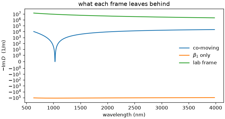
The lab frame carries the whole of \(\beta\), about \(10^7\ \mathrm{m^{-1}}\). Removing the group delay takes five orders of magnitude off it, and removing \(\beta_0\) as well leaves only the group-delay dispersion and the third-order term — a few tens of inverse metres, and zero at the carrier by construction. That cancellation is also the accuracy limit of the assembly: five digits of \(\beta\) are lost to it, so a comparison of two implementations of the operator is best stated against \(\beta\) rather than against D.

The carrier frame’s pointer above comes from SEP 35.