Antiresonant tube-lattice fibres

Use a tube-lattice model when resonances in a ring of glass tubes govern the loss and dispersion. The model supplies fitted propagation constants while retaining capillary-like core fields. Read its geometry and wavelength limitations before using it to predict a dispersive-wave wavelength or a compression length.

Antiresonant tube-lattice fibres: the Vincetti model

VincettiMode describes a single-ring antiresonant hollow-core fibre: a hollow core surrounded by one ring of glass tubes, which guides by antiresonant reflection from the tube walls. It is a Marcatili mode whose index and loss are corrected by published fits; the field, the gas fill and the loss policy are the capillary’s. The core radius is \(a\), each tube has outer radius \(r\) and wall thickness \(t\), and there are \(N\) tubes. The clear gap between adjacent tubes is \(\delta=2[(a+r)\sin(\pi/N)-r]\). A negative gap means overlapping tubes and is refused, including at a taper’s breakpoints; touching tubes are accepted. TubeLattice stores these fixed tube dimensions, and tube_gap(), core_radius_from_gap() and tube_radius_from_gap() convert between gap, core radius and tube radius.

from solprop.constants import C
from solprop.modes import TubeLattice, VincettiMode
import numpy as np

lattice = TubeLattice(wall_thickness=180e-9, tube_radius=9e-6, n_tubes=6)
mode = VincettiMode(15e-6, "Ar", 1.0, lattice=lattice)
omega = np.array([2 * np.pi * C / 800e-9])
index = mode.neff(omega)
fitted_area = mode.effective_area(omega)  # frequency-dependent fit, m^2
propagation_area = mode.aeff()  # Marcatili field integral, m^2

To propagate, pass lattice= beside an integer modes= to prop_capillary or Simulation.from_capillary, or build a numbered set with ModeCollection.vincetti. Supplied mode objects carry their own geometry, so combining them with lattice= is refused. The antiresonant tutorial shows argon pressure tuning and a short Kerr propagation.

The model combines the confinement-loss fits of Vincetti (2016) and Vincetti and Rosa (2019) with the dispersion fit of Rosa, Melli and Vincetti (2021). These are empirical fits, not an exact solution of Maxwell’s equations for the tube geometry. Every coefficient was transcribed from the papers and checked term by term against the published text. The minimum-loss prefactor is the 2019 paper’s \(3\times10^{-4}\), the minimum, rather than the 2016 paper’s average \(5\times10^{-4}\). The 2016 equation (its Eq. 3) has been checked against the typeset page and matches term for term, apart from the prefactor; the paper’s normalised-loss definition carries an extra \(\sqrt{r/\lambda}\) that would make it inconsistent with Eq. 3, which is the dimensionally consistent form and the one used. In five places the printed papers and earlier published implementations of the model differ; the form solprop uses is decided below, term by term.

With \(\lambda=2\pi c/\omega\), tube index \(n_t=\operatorname{Re}n_{\rm cladding}\), and gas index \(n_g\) from the declared mixture, the normalised wall frequency is \(F=(2t/\lambda)\sqrt{n_t^2-n_g^2}\): the resonance of a wall of index \(n_t\) in a core of index \(n_g\) is \(k t\sqrt{n_t^2-n_g^2}=q\pi\), so the resonances move with the fill, by \(-0.24\,\%\) in wavelength at 10 bar argon and \(-0.7\,\%\) at 30 bar. Tube resonances occur at the fitted HE and EH cutoff frequencies \(F_c(\mu,\nu)\) of the 2019 paper, equations 4–5. Each contributes a Lorentzian \(L(x)=\gamma_l^2/(\gamma_l^2+x^2)\), with \(\gamma_l=0.003\) and weight \(A(\mu)=2000\exp[-0.05|\mu-1|^{2.6}]\). The loss in dB/m is

\[\begin{split} \begin{aligned} CL_{\min}&=3\times10^{-4}\frac{\lambda^{4.5}}{a^4} (1-t/r)^{-12}\frac{\sqrt{n_t^2-1}}{t\sqrt r} \exp\left[\frac{2\lambda}{r(n_t^2-1)}\right],\\ CL&=CL_{\min}\sum_{\nu=1}^{n_{\rm terms}}\sum_{\mu=1}^{n_{\rm terms}} A(\mu)\left[L(F-F_c^{HE})+L(F-F_c^{EH})\right]. \end{aligned} \end{split}\]

The default is eight terms in each sum. The papers truncate only the azimuthal sum, at \(\mu\le8\); solprop applies the same count to \(\nu\) and refuses more. The EH cutoff fit carries \(1/(7.75-\nu)\), whose pole lies between the seventh and the eighth term, so the eighth term is already past it; it is harmless in practice, since it sits at \(F\approx7\) (about 54 nm for 180 nm walls). The minimum loss keeps its printed \(n_t^2-1\) factors: the 2016 fit is the evacuated one, and filling them changes \(CL\) by \(-0.9\,\%\) at 30 bar. The power attenuation coefficient is \(\alpha=CL\ln(10)/10\) and the confinement contribution to the imaginary index is \(c\alpha/(2\omega)\). loss=True, False, a nonnegative scale, and an absolute callable \(\alpha(\omega)\) have the same meaning as for a capillary. A scale is a user adjustment to the fit. Gas absorption retains the parent’s material contract.

The real-index fit uses an effective core radius and a dispersive resonance term:

\[\begin{split} \begin{aligned} R_{\rm eff}&=\left[1.027+10^{-3}(F+2/F^4)\right] \sqrt{a^2+\frac N\pi\frac3{64}r^2 \left[1+(3+10\lambda/a)\delta/r\right]},\\ L_i(F,F_0)&=\frac{F_0^2-F^2}{(F^2-F_0^2)^2+(0.03F)^2},\\ \Delta n&=4.5\times10^{-7}(1-t/r)^{-4}(\lambda/a)^2 A(1) \sum_{\nu=1}^{n_{\rm terms}} [L_i(F,F_c^{HE}(1,\nu))+L_i(F,F_c^{EH}(1,\nu))],\\ \operatorname{Re} n_{\rm eff}&=n_g- \frac1{2n_g}\left(\frac{u_{nm}c}{\omega R_{\rm eff}}\right)^2+\Delta n. \end{aligned} \end{split}\]

The square on \(r\) follows from the trapezoid area in the geometric derivation. The waveguide term is the first-order expansion of \(\beta=\sqrt{n_g^2k^2-(u_{nm}/R_{\rm eff})^2}\), one power of \(n_g\), as the parent’s full model has it; the neglected second order is \(1.6\times10^{-8}\) at 800 nm in a 15 µm core. neff_minus_one forms refractivity directly, preserving small gas contributions. The inherited evanescent floor clamps the real index and zeros its derivative where it binds. model="reduced" is refused: this class already selects a specific model.

The transverse field, normalisation and protocol aeff(z) are Marcatili’s: the fits describe the index and the loss, not the field. The separately exposed fitted area is

\[A_{\rm eff}(\omega,z)=\frac{0.48}{8\pi n_g} \frac{(u_{nm}\lambda)^2}{n_g-\operatorname{Re}n_{\rm eff}}.\]

Away from resonance it reduces to \(0.48\pi R_{\rm eff}^2\), independent of the fill, \(0.48\pi\) being Marcatili’s HE₁₁ area factor; the FEM area at 10 bar argon is fill independent to \(10^{-4}\). It can diverge or become negative near a resonance where the fitted denominator changes sign. It is a diagnostic fit and does not replace the positive field integral used by the nonlinear transform or the area stored in output metadata.

The five conventions

Earlier published implementations of the Vincetti model (pyJCMwave among them) share one form of the fits; the printed papers give another. One rule decides each term: a principled physical reason first; else, if the effect against the finite-element data is negligible, the printed form; else the form that fits the finite-element data best. The finite-element data are converged solutions for a six-tube fibre, evacuated and at 10 bar of argon (below). The size of each change is given for the tutorial fibre (15 µm core, 180 nm walls, 9 µm tubes, six of them) in argon at 294 K, as solprop’s form minus the earlier one.

term	solprop	earlier implementations	printed	reason	size
dispersion width \(\gamma_d\)	0.03	0.03	0.003 (2021 eq. 2)	best FEM fit: the near-resonance index is 3.2× (vacuum) and 2.3× (argon) worse with 0.003	none
\(R_{\rm eff}\) coefficient	\(3+10\lambda/a\)	20	\(3+2\cdot10\lambda/R_{co}\), that is 20 (2021 eq. 10, typeset); Melli et al. 2025 eq. 7 writes 20	negligible (0.9 % of the decrement, a quarter of the fit’s median residual); solprop’s 10 came from a misreading of the printed bracket and is kept for now, with the vacuum index RMSE 13 % better than with 20	\(n_{\rm eff}\) \(-1.7\times10^{-6}\) at 800 nm; \(\beta_2\) \(-7.7\) fs²/m (1.7 %) at 800 nm, \(+2.2\) at 1030 nm; area \(-1.0\,\%\)
waveguide decrement	\(D_0/n_g\)	\(D_0/n_g^2\)	\(D_0/n_g\) (2021 eqs. 21, 23)	physical: the expansion of \(\beta\); the FEM’s 10 bar index is predicted from its vacuum index to \(2.2\times10^{-8}\) with one power and \(6.7\times10^{-7}\) with two	30 bar: \(n_{\rm eff}\) \(-1.3\times10^{-6}\) at 800 nm; \(\beta_2\) \(+0.1\) fs²/m at 800 nm, \(+8.9\) (1.7 %) at 1030 nm
area prefactor	\(1/n_g\)	none	\(1/n_g\) (2021 eq. 22)	physical: with the single-power decrement the area is fill independent, as the FEM’s is to \(10^{-4}\)	30 bar: area \(-0.8\,\%\)
normalised frequency	\(\sqrt{n_t^2-n_g^2}\) wherever \(F\) enters	\(\sqrt{n_t^2-1}\)	\(\sqrt{n_t^2-n_g^2}\) (2021 eq. 23)	physical: the wall’s slab resonance in the filled core	30 bar: the \(q=1\) loss peak 2.5 nm shorter (0.08 nm at 1 bar); loss ×0.74 at 400 nm, ×1.01 at 800 nm; \(\beta_2\) \(+71\) fs²/m (1.3 %) at 400 nm, \(+2.4\) at 800 nm

All five together at 30 bar: \(n_{\rm eff}\) \(-3.0\times10^{-6}\) and \(\beta_2\) \(-4.9\) fs²/m at 800 nm (where \(\beta_2=+74\) fs²/m), \(+70\) fs²/m at 400 nm, area \(-2.4\,\%\); at 1 bar \(-1.7\times10^{-6}\), \(-7.7\) fs²/m at 800 nm, \(+36\) at 400 nm, area \(-1.0\,\%\). Evacuated, only the radius coefficient acts. The earlier form can be assembled from the same code as solprop.modes.antiresonant.LEGACY_CONVENTIONS, which the tests use to compare with earlier implementations and which no propagation uses; solprop’s own form is checked against an independent symbolic derivation and the finite-element rows.

The 2019 validation geometries span \(0.05\le t/r\le0.2\), \(6\le N\le10\), tube indices 1.44–2.42 and the first four transmission bands. Those are sampled geometries, not a proven domain of validity, and no range of the normalised frequency \(F\) is taken as one either. Construction logs once for geometry outside the stated ranges, and once for a non-HE11 mode: higher orders retain their own Bessel zero and field, but the loss and dispersion corrections are fundamental-mode fits. Frequency excursions are not warned about on every evaluation. The thin-wall 30 micrometre example below extrapolates \(t/r=0.02\) and logs that fact.

Accuracy against a finite-element solution

The model is compared with converged finite-element (FEM) solutions of one fibre: a 30 µm core (15 µm radius) with 180 nm walls and six tubes of outer radius 10.38 µm, a \(t/r=0.017\) fibre outside the fits’ validated 0.05–0.2. The FEM data cover 79 wavelengths from 200 to 1500 nm evacuated and 20 from 355 to 946 nm at 10 bar of argon and 293 K. The comparison uses the FEM’s own silica index (without absorption) and the same three-pole argon Sellmeier fit (solprop’s kingston source, whose gas indices match the FEM’s exactly). No parameter was refitted.

With the conventions above, the index residual has RMSE \(7.5\times10^{-6}\) over the 79 vacuum rows and, away from the resonances, a median of 2.9 % of the waveguide decrement (p90 12 %, maximum 26 %); at 10 bar \(4.5\times10^{-6}\) and 0.7 %, and the vacuum-to-argon change of the index is reproduced to \(7\times10^{-8}\). The loss in the interior of the first window is 0.5–1.6 times the FEM’s; at the band edges the fit’s Lorentzians are far narrower than the FEM resonances and the loss is up to 150 times too low. The fitted area’s median residual is 2.5 % (vacuum) and 1.2 % (argon) away from resonance.

The group-velocity dispersion is the quantity this model is used for, and it is where the fit is weakest. In the first transmission band of this fibre the FEM’s own \(\beta_2\) is more negative than the model’s by 1 % at 607 nm, 18 % at 782 nm, 48 % at 913 nm and 70 % at 1013 nm in vacuum (\(-1268\) against \(-744\) fs²/m), and by 24–67 % over 720–913 nm at 10 bar. It is the curvature of the model’s U-shaped index residual (+24 % of the decrement at 400 nm, about zero at 800 nm, +5 % at 1360 nm), not a differencing artefact, and none of the five conventions moves it by more than 2 %. The 2019 and 2021 fits were validated for \(t/r\) between 0.05 and 0.2; this fibre lies outside that range, and so does the tutorial’s. These numbers are pinned as a regression test in tests/modes/test_vincetti_fem.py.

The frequency derivative is analytic, including tube-index-dependent exponents and both material derivatives; the gas index enters \(F\) and the decrement, and its slope comes with it. An independent symbolic derivation of the model agrees within 1.1e-12 relative (bound 1e-10), and the contour-integral check within 8.7e-15 (bound 1e-11). beta2 is the common finite difference of the analytic beta1; near a resonance, where the index curves sharply, its difference error is larger. Radius and density are the same parameter paths as a capillary’s, giving a constant operator for a constant fill and a Chebyshev expansion along z, which every backend executes, for a gradient.

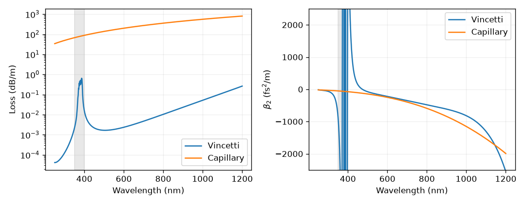
Evacuated 30 micrometre core, 180 nm walls, 9 micrometre outer tube radius and six tubes, against the same-radius capillary. The shaded interval is the nominal first wall-resonance band (350–400 nm), not a validity boundary. Both curves use the default silica material.