Profiles along the fibre

A pressure gradient, a taper, a pre-ionised section: each describes a physical quantity that changes along the propagation axis. solprop represents such a quantity as a scalar path, giving its value, derivative and any breakpoints as functions of position \(z\). Everything on this page lives in solprop.profiles, apart from the steady-flow builder of solprop.gasflow.

Most runs never build a path by hand: pressure=(p_in, p_out) on prop_capillary or prop_waveguide builds the steady flow of the gas through the guide’s own bore, with a choked vacuum end, and temperature= or a radius given as a path does the rest. This page is for readers who want to know what those fills are — the laminar flow law, the choked end, the numerical floor, the limits of the flow regime, a temperature that varies along the fibre, and how a pressure becomes a number density — or who need to declare a path of their own.

The paths

class	shape	breakpoints
Constant	one value everywhere	none
Linear	a taper between two ends, clamped outside	both ends
PiecewiseLinear	linear between stages, clamped outside	every stage
PressureGradient	steady flow, in bar, following the bore if given	every stage, and the radius’s kinks
DensityPath	number density under a pressure path	the pressure path’s
FromCallable	anything, with declared breakpoints	as declared

Pressures are in bar at this interface, the one documented departure from SI at the user interface (conventions, §1). Positions are in metres and densities in m⁻³.

Paths compose. Scaled(path, factor) multiplies values and derivatives; Sum(paths) adds them in order and takes the union of breakpoints and spans. These compose the partial-pressure, total-density and Kerr paths of gas mixtures. DensityPath accepts a custom Species as well as built-in gas names, using that species’ equation of state. It continues endpoint densities outside the declared span, refuses negative pressures at declared boundaries and floors negative interpolant overshoot between them.

What a path has to provide, and why

The cumulative linear operator \(\Phi(\omega, z) = \int D\,\mathrm{d}z\) is built by resolving the scalar parameter paths first and taking the union of the interval edges they produce as the mandatory split of the expensive array-valued operator (solprop.translate.chebyshev.build_from_paths(), stepper design, §4). That fixes the interface:

Vectorised evaluation. The adaptive builder samples at Chebyshev points in blocks, so path(z) takes an array of positions and returns an array of values.

Declared breakpoints. The adaptive split finds smooth structure by bisection, but it cannot see a kink it was not told about, and a step must land exactly on one rather than straddling it. Every stage boundary of a fill is therefore a breakpoint, declared, not discovered.

An analytic derivative, or an honest declaration. derivative_is_analytic says which, so a caller can tell a converged quantity from a differenced one. It matters because a differenced derivative floors the whole table at about \(10^{-8}\), while the co-moving frame needs \(\beta_1\) to about \(10^{-10}\).

A profile is directly usable as a path — build_from_paths([profile], ...) works through __call__ — and the caller passes the union of the profiles’ breakpoints as the mandatory edges.

Steady-flow fills

A hollow fibre between two gas cells carries a steady flow from the high-pressure cell to the low one. Along a bore narrow enough for the flow to be laminar, the velocity profile is Poiseuille’s, and the mean velocity is

\[\bar u(z) = -\frac{a(z)^2}{8\eta}\,\frac{\mathrm{d}p}{\mathrm{d}z},\]

with \(a\) the core radius and \(\eta\) the gas viscosity. For an isothermal ideal gas the mass density is proportional to \(p\), so the mass flow is

\[\dot m \propto p\,\bar u\,\pi a^2 \propto -\frac{a^4}{\eta}\,p\,\frac{\mathrm{d}p}{\mathrm{d}z} = -\frac{a^4}{2\eta}\,\frac{\mathrm{d}(p^2)}{\mathrm{d}z},\]

and in a steady state it is the same everywhere between two cells. Hence \(p^2\) is linear not in \(z\) but in the hydraulic resistance \(R(u, v) = \int_u^v a^{-4}\,\mathrm{d}z\). Between two stage ends \(z_i\) and \(z_{i+1}\), held at fixed pressures by the cells,

\[p(z)^2 = (1 - f)\,p_i^2 + f\,p_{i+1}^2, \qquad f(z) = \frac{R(z_i, z)}{R(z_i, z_{i+1})}, \qquad \frac{\mathrm{d}p}{\mathrm{d}z} = \frac{(p_{i+1}^2 - p_i^2)\,a(z)^{-4}}{2\,R(z_i, z_{i+1})\,p}.\]

This is eq. (6) of Pennetta et al., APL Photonics 4, 056105 (2019), applied to each stage, every one an independent flow between two cells. With a constant radius \(f = (z - z_i)/(z_{i+1} - z_i)\), and the fill is the familiar uniform law

\[p(z) = \sqrt{p_i^2 + \frac{z - z_i}{z_{i+1} - z_i}\left(p_{i+1}^2 - p_i^2\right)},\]

which is what PressureGradient computes when it is given no radius or a constant one, exactly. Given a varying radius (PressureGradient.from_stages(positions, pressures, radius=...), or through the simulation constructors, which pass the guide’s own), the fill follows the bore: a narrow waist carries most of the pressure drop and decouples the two ends.

Both forms are evaluated as the convex combination \((1 - f)\,p_i^2 + f\,p_{i+1}^2\), which cannot cancel. The textbook arrangement \(p_i^2 + f\,(p_{i+1}^2 - p_i^2)\) does cancel when a fill runs down into a floor far below its start: into a floor \(10^{-4}\) of the start it errs by a few parts in \(10^9\) and dips below its own end pressure. The derivative is exact: it needs the weight \(a^{-4}\) itself, never the radius’s slope. The resistance is integrated in closed form where the radius is linear,

\[\int_{z_0}^{z} a^{-4}\,\mathrm{d}z' = \frac{(z - z_0)\,(a_0^2 + a_0 a + a^2)}{3\,a_0^3 a^3},\]

a form with no subtraction, and otherwise by a Chebyshev interpolant of \(a^{-4}\) on each interval between the radius’s and the stages’ breakpoints, integrated exactly once its last coefficients fall below \(10^{-13}\) of the largest (a radius that has not converged by degree 256 has an undeclared kink and is refused by name). The fill’s breakpoints are the union of the stage positions and the radius breakpoints inside it. hydraulic_integral() returns \(R\) per stage.

Stage positions must be strictly increasing; an unsorted stage table is refused at construction, since it would otherwise interpolate the wrong stage without complaint.

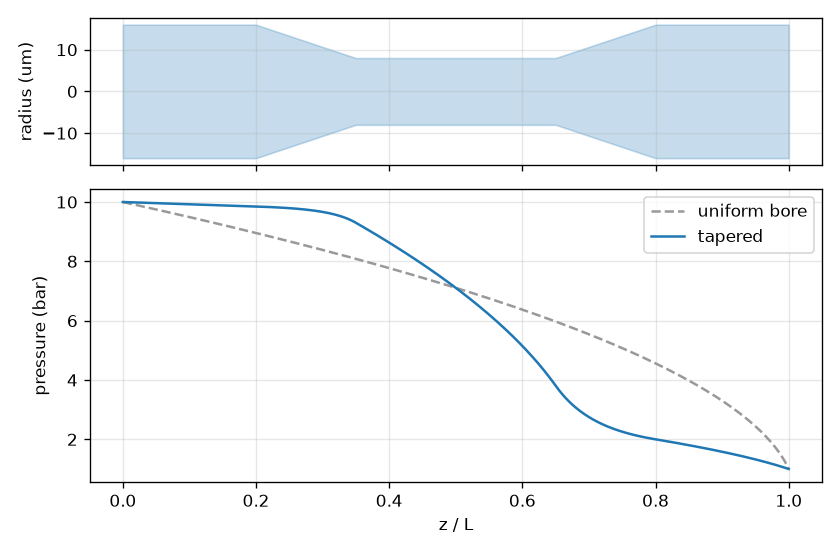
Steady flow of 10 bar to 1 bar through a uniform bore (grey) and through a fibre with a linear down-taper, a narrow waist and a linear up-taper (blue), after Pennetta et al. (2019), Fig. 5(b). The waist carries almost the whole pressure drop: the gas before it stays near the entrance pressure and the gas after it near the exit’s.

A vacuum end is choked

A fibre exhausting into a pumped chamber cannot carry more than the gas can leave at the speed of sound: the throughput at the exit is bounded by \(p_e\,\pi a_e^2 c\). The laminar PV throughput of the last stage is

\[Q = \frac{\pi\,(p_h^2 - p_e^2)}{16\,\eta\,R},\]

with \(p_h\) the stage’s other end and \(R\) its resistance (\(L/a^4\) for a uniform bore). Equating the two, as the HiSol.jl design tool does,

\[k\,(p_h^2 - p_e^2) = p_e, \qquad k = \frac{1}{16\,\eta\,c\,a_e^2 R}, \qquad p_e = \frac{2 k p_h^2}{1 + \sqrt{1 + 4 k^2 p_h^2}}.\]

This root does not cancel when \(k p_h \ll 1\), the usual case, where it tends to HiSol’s \(k p_h^2 = D^2 p_h^2/(64\,\eta L c)\); HiSol drops \(p_e^2\) and solprop does not need to. A 5 m nitrogen capillary of 500 µm core diameter fed at 4.2 bar chokes at 224 mbar; a 1 m argon fibre of 30 µm core diameter at 20 bar at 79 mbar; a 3 m helium capillary of 250 µm core diameter at 5 bar at 41 mbar.

solprop.gasflow.steady_fill() builds a fill from the gas, the stage table and the bore, and each outer end that is the low end of its stage takes \(\max(\text{declared}, \text{choked}, \text{floor})\). A declared zero replaced by the choked value is logged at INFO; a nonzero declared pressure raised to it is logged as a WARNING naming both, because the chamber may well be at the declared pressure — the fibre end cannot be. Interior stage pressures are never choked (the chamber between two fibres is not modelled). The simulation constructors do this by default for any circular hollow guide (capillary, Vincetti or tabulated hollow modes). With vacuum_end="floor" the declared end pressures are kept instead, subject only to the numerical floor described below; this concerns the ends only, and a taper’s fill still follows the bore (for a uniform bore it is exactly the uniform law). Every mode that declares a core_radius — every MarcatiliMode subclass, a TabulatedMode built from arrays included — is taken as a circular bore of that radius. Mixture.fill takes the same radius= and vacuum_end=; without a radius it keeps the uniform law and the floor, since the choke needs the bore.

How good is the estimate? The test suite integrates the one-dimensional steady compressible laminar flow — continuity, momentum with the acceleration term, Poiseuille wall friction — from the fed end until the flow chokes, with an isothermal wall and, separately, an adiabatic one. The Poiseuille mass flow agrees with both to 2–4 %: the acceleration term matters only near the exit. The exit pressure depends on where the flow chokes: an isothermal wall chokes at the isothermal sound speed \(c/\sqrt\gamma\), and the closed form with that speed matches it to 2–3 %; an adiabatic wall chokes where the gas has cooled. solprop’s closed form uses the adiabatic \(c\) at the fill temperature, as HiSol does, and lies between the two walls: the isothermal integration is 16–25 % above it and the adiabatic one 10–16 % below it, for Gebhardt et al.’s nitrogen capillary (500 µm, 5 m, 4.2 bar) and an argon down-taper (125 µm to 75 µm over 1 m, 5 bar). A real capillary is close to isothermal along most of its length and not at the exit: microtube experiments show near-isothermal flow upstream and a quasi-adiabatic exit, which points to the adiabatic wall’s value, about \(\sqrt{2/(\gamma+1)}\) times the closed form. For a nonlinear optics run the difference is a few per cent of a residual pressure that is itself a few per cent of the entrance’s.

The numerical floor

Look at \(\mathrm{d}p/\mathrm{d}z\) as \(p \to 0\): it diverges. A gradient that ends at exactly zero pressure therefore has an infinite slope at that end. The usual smooth-coefficient assumptions behind a method’s convergence order no longer hold. The measured order depends on the configuration; the RDW study shows a particularly strong reduction. Nothing in the run reports this reduction, so check convergence of the observable rather than interpreting a local tolerance as a global error bound.

A choked end is far from zero. Where a fill is built without the gas or the bore — a PressureGradient constructed directly, a Mixture.fill without a radius, or vacuum_end="floor" — any stage pressure below the floor is raised to it and the substitution is logged, naming the position and the reason:

pressure fill raised from [0.0] bar to the floor 8.000e-05 bar at z = [1.5] m:
dp/dz diverges at a true vacuum end, which caps every integration scheme at about
third order (docs/dev/stepper.md section 10, trap 5). Pass floor= to choose another value.

The default floor is \(10^{-4}\) of the highest stage pressure, so it means the same thing for a 0.8 bar gradient as for a 40 bar one. At that level the residual gas contributes \(10^{-4}\) of the fill’s refractivity while the slope stays finite and cheap for the adaptive split to resolve. Pass floor= to choose another value; floor=0.0 keeps the true vacuum end, for comparison with a calculation that has one, and logs a stronger warning. Such a comparison also needs vacuum_end="floor", since a choked end is not a vacuum.

Note

One more degenerate case is refused at construction rather than returning NaN: a fill whose highest pressure is below about \(10^{-154}\) bar squares to zero and collapses the whole profile to \(0/0\).

Flow regime

The laminar law is a model with limits on both sides, and steady_fill() checks both through a FlowReport (also available from flow_report() for any fill).

Reynolds number. \(Re = 4\dot m/(\pi d \eta)\), which is Gebhardt et al.’s \(4 M Q/(R T \pi d \eta)\) written with the mass flow. The mass flow is constant along a stage, so in a taper the waist has the largest Reynolds number. Gebhardt et al., Opt. Express 29, 6957 (2021), measured spatio-temporal instabilities of the output beam of differentially pumped capillaries that set in at \(Re \approx 2040\) — where pipe flow starts to sustain turbulent puffs (Avila et al., Science 333, 192 (2011)) — and were worst near 2400, and recommend \(Re < 2000\) (their eq. 4: 3.75 bar for a 5 m, 500 µm nitrogen capillary; solprop’s own number is within 1 % of it). Above REYNOLDS_LAMINAR_LIMIT \(= 2000\) the fill warns (GasFlowWarning) with the peak and its position. The laminar fill is not valid there; the warning does not replace it with a turbulent one. A short fibre carrying a large pressure difference is often far above the limit — a millimetre of capillary between 2 bar and 1 bar is at \(Re \sim 10^4\).

Knudsen number. \(Kn = \lambda/d\), with the viscosity-based mean free path \(\lambda = (\eta/p)\sqrt{\pi k_B T/(2m)}\) (mean_free_path()). First-order wall slip raises a tube’s throughput to \(Q_\mathrm{Pois}\,[1 + 8\,Kn(\bar p)]\), with \(\bar p = (p_h + p_l)/2\) the stage’s mean pressure, so a stage whose Knudsen number at \(\bar p\) and at its narrowest diameter exceeds KNUDSEN_SLIP_LIMIT \(= 0.01\) has a laminar throughput, Reynolds number and choked pressure off by ten per cent or more, and the fill warns. Above KNUDSEN_TRANSITION_LIMIT \(= 0.1\) the gas is transitional between continuum and molecular flow; the fill also warns if more than TRANSITIONAL_COLUMN_LIMIT \(= 1\,\%\) of a stage’s column density \(\int p\,\mathrm{d}z\) lies there. Otherwise it logs, at INFO, each stage’s exit Knudsen number and the length over which \(Kn > 0.1\). A choked helium exit is transitional, but only just before the end: a capillary of 125 µm core radius filled with helium from 1.2 bar to vacuum over 1 m chokes at 7.1 mbar with \(Kn = 0.11\), transitional over its last 6 µm; the same capillary from 0.8 bar over 1.5 m chokes at 2.1 mbar with \(Kn = 0.36\), transitional over 0.13 mm holding a millionth of the gas. Neither warns. A nitrogen-filled bore of 5 µm radius between 50 and 30 mbar, with \(Kn(\bar p) = 0.16\), does. The FlowReport carries each stage’s peak, exit and mean-pressure Knudsen numbers and the transitional length and column share.

The viscosities, heat capacities and mixing rules behind these numbers are in solprop.physdata.transport: CoolProp’s dilute viscosity where it has a model, and a table from the NIST Chemistry WebBook for Ne, Kr, Xe, D₂ and N₂O, both over 200–600 K (SF₆ from 225 K, N₂O to 500 K; a temperature outside is refused). Mixtures use Wilke’s rule, which is checked here only to reduce to the pure gas and to reproduce CoolProp’s air viscosity from nitrogen and oxygen within 0.3 %; its documented accuracy is 1–2 %.

A temperature that varies along the fibre

The laminar law above assumes one temperature. A fibre heated or cooled along its length — a hot section in an oven, a cell at another temperature — carries a gas whose temperature \(T(z)\) follows the wall’s: the flow is slow and the bore narrow, so the gas takes the wall temperature, and solprop takes \(T(z)\) as prescribed (no energy equation is solved). Pass it as a ZProfile wherever a temperature is taken: temperature= of prop_capillary, prop_waveguide, the simulation constructors, fill(), steady_fill() and the gas-filled modes.

The mass density of an ideal gas is \(pM/(RT)\), so the Poiseuille mass flow becomes

\[\dot m = -\frac{\pi a^4}{8\,\eta(T)}\,\frac{p M}{R T}\,\frac{\mathrm{d}p}{\mathrm{d}z} = -\frac{\pi M}{16 R}\,\frac{a^4}{\eta(T)\,T}\,\frac{\mathrm{d}(p^2)}{\mathrm{d}z},\]

still constant along a stage, and \(p^2\) is linear in the weighted resistance \(W(u, v) = \int_u^v w\,a^{-4}\,\mathrm{d}z\) with the flow weight

\[w(z) = \eta\big(T(z)\big)\,T(z).\]

Everything above holds with \(a^{-4}\) replaced by \(w\,a^{-4}\): the fraction \(f = W(z_i, z)/W(z_i, z_{i+1})\), the analytic slope \(\mathrm{d}p/\mathrm{d}z = (p_{i+1}^2 - p_i^2)\,w\,a^{-4}/(2 W p)\), and the breakpoints, which include the temperature’s. A constant factor in \(w\) cancels from \(f\), so a constant temperature is the law above, bit for bit. temperature_weight() builds \(w\): the gas’s viscosity (solprop.physdata.transport, Wilke’s rule for a mixture) as a Chebyshev series in \(T\) over the temperatures the path takes on the fill, accepted once it reproduces direct calls to \(10^{-6}\) relative on a check grid between its nodes (three thousand times below the transport data’s own 0.3–3 %; CoolProp’s helium viscosity is not smooth enough for a tighter tolerance, and every built-in gas meets this one over its whole declared range by degree 64), times \(T\), evaluated on the path as a SeriesOfPath; PressureGradient stores it as its weight and integrates \(w\,a^{-4}\) by a converged Chebyshev interpolant on each interval, as it does a smooth radius. A gradient under a temperature path is weighted with or without a radius (Mixture.fill without one keeps the uniform bore but not a uniform temperature), which needs the gas’s transport data: a custom species is refused by name.

A PressureGradient supplied beside a temperature path — to Mixture.fill, partial_pressures, a gas-filled mode or a constructor — must carry the weight of this gas and this temperature path: every door compares its weight with the one the declaration implies (normalised, to \(10^{-5}\)) and refuses a missing or foreign weight by name. Any other pressure profile (a Linear, a PiecewiseLinear, a callable) makes no flow claim and is taken as the declared pressure. A retained weighted fill is refused by Mixture.with_fill(fractions), which asks for the pressure again so that the flow is rebuilt for the new composition.

The rest of the flow follows the local state. A choked end equates the stage’s mass flow to the sonic one at its own temperature \(T_e\), \(\pi M (p_h^2 - p_e^2)/(16 R W) = p_e M \pi a_e^2 c_e/(R T_e)\), so

\[k = \frac{T_e}{16\,c_e\,a_e^2\,W}, \qquad c_e = c(T_e),\]

which is \(1/(16\,\eta c a_e^2 R)\) at a constant temperature; a warm exit chokes lower. The Reynolds number \(2\dot m/(\pi a\,\eta(T))\) takes the local viscosity and the Knudsen number the local mean free path; the mean-pressure Knudsen number takes the largest \(\lambda(1\,\text{bar}, T)/d\) on the stage. A stage’s PV throughput is quoted at its low end’s temperature, \(Q = \pi T_e (p_h^2 - p_l^2)/(16 W)\), which is where the FlowReport records it (StageFlow.temperature); the report’s viscosity and sound_speed are the values at the fill’s first position.

What this does not model: the gas is ideal in the flow law (the density along the fill is real-gas); heat conduction along the gas and viscous heating are ignored, so the wall’s \(T(z)\) is the gas’s; and the rotational Raman populations do not follow \(T(z)\) (Raman).

Density along a fill

DensityPath turns a pressure path into a number density. density() is a real-gas call into optmat’s equation of state that is costly per call and is not vectorised, while the Chebyshev builder samples a path thousands of times, so the equation of state is evaluated once on a fine pressure grid spanning the path’s range and interpolated with a cubic spline. Its derivative is exact, so

\[\frac{\mathrm{d}\rho}{\mathrm{d}z} = \rho'(p)\,\frac{\mathrm{d}p}{\mathrm{d}z}\]

stays analytic whenever the pressure path is. The spline reproduces direct calls to better than \(10^{-9}\) relative, which is far tighter than the equation of state’s own accuracy.

Under a temperature path the density is \(\rho\big(p(z), T(z)\big)\), a function of two variables. Tabulating it the same way would cost a thousand equation-of-state calls per temperature; instead the compressibility factor \(Z = p/(\rho k_B T)\), which separates the ideal-gas dependence from the real-gas correction, is tabulated as a tensor Chebyshev series over the rectangle of pressures and temperatures the two paths span, each axis raised from degree 8 until its last coefficients fall below \(10^{-13}\) of the largest. \(Z\) is analytic and close to one for most fills (at 294 K and 40 bar it is 1.02 for helium and 0.98 for argon), but not for the heavy gases at high pressure: xenon reads 0.94 at 10 bar and 0.73 at 40 bar. Then

\[\rho = \frac{p}{k_B T\,Z}, \qquad \frac{\mathrm{d}\rho}{\mathrm{d}z} = \rho_p\,p' + \rho_T\,T', \qquad \rho_p = \frac{1 - p Z_p/Z}{k_B T Z}, \quad \rho_T = -\rho\left(\frac1T + \frac{Z_T}{Z}\right),\]

with the series’ exact partial derivatives, so the ideal-gas part is exact and the derivative analytic. For argon from 10 bar to 0.5 bar and 294 K to 380 K the table is \(9 \times 17\) nodes — 234 calls with the degree trials, against the 1024 of the constant-temperature spline — and reproduces direct calls to better than \(10^{-12}\); the tests assert \(10^{-9}\) for helium, nitrogen, argon and xenon. The nodes are Chebyshev points of the first kind, which never fall on a zero-pressure end. A constant temperature — a number or a constant path — takes the spline above, bit for bit.

A fill that reaches 0 bar, such as Linear(1.5, 0.0, L) or a stage ending at 0 bar, has a density of exactly zero there. Its table along z is exactly zero at that end too. The fit alone would miss the zero by a few ulp of the density scale, of either sign, and a negative density is refused at translation. A square-root vacuum end, from a steady-flow gradient to pressure_floor=0.0, is not changed: its table is positive at the end, by about \(10^{-8}\) of its scale.

A worked example

A typical resonant-dispersive-wave fill is a helium gradient from 0.8 bar to vacuum over 1.5 m in a 125 µm capillary. Built directly, without the gas or the bore, the vacuum end is floored rather than choked (through prop_capillary(..., "He", (0.8, 0.0)) it would choke at 2.1 mbar instead, above):

from solprop.physdata import Gas
from solprop.profiles import DensityPath, PressureGradient

fill = PressureGradient.two_point(1.5, 0.8, 0.0)  # logs the floor substitution
density = DensityPath(Gas.He, fill)

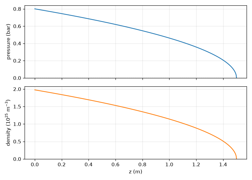
A helium gradient from 0.8 bar to vacuum over 1.5 m, and the number density that follows it. The pressure falls as a square root, so the density does too: a third of the gas is in the first quarter of the fibre and half in the first 37 %. The dashed line is the floor the vacuum end was raised to, which is invisible on a linear axis and is the point.

Where solprop’s choices differ from Luna.jl’s, the differences are listed in Noteworthy differences from Luna.

Related calculations

The tapered-capillary example follows a changing bore; the RDW lesson uses a pressure gradient. Continue to mode conversion when the local modes change shape, and to the gradient-compressor example for a full comparison.