Varying operators and interpolation accuracy#
A varying pressure or geometry changes dispersion along the propagation. Solprop approximates the required operator with controlled tables, then integrates the represented function. This chapter explains table tolerance, parameter expansions and handling of profile boundaries. Start with linear propagation and moving frames for the physical operator and sign conventions.
Cumulative operator#
\(\Phi(\omega, z)\) has two representations. The one a capillary gets is the expansion in
the scalar parameters (below); the general one, and the fallback for
everything else, is a piecewise Chebyshev polynomial in z with array-valued
coefficients, built by solprop.translate.chebyshev.build() and returned as a
solprop.translate.chebyshev.PiecewiseChebyshev. Both are evaluated through
solprop.translate.linop.delta_phi() and
solprop.translate.linop.unitary_phase() and nothing downstream can tell them apart.
The z table is described first because the expansion is built out of its machinery.
On interval \(i\) spanning \([z_i, z_{i+1}]\),
with the coefficients held in one rectangular array of shape (n_intervals, n_deg, ...),
the trailing axes being those of the value; for the kernel contract that value is
(n_batch_or_1, n_modes, n_pol, n_omega). Intervals that need a lower degree carry
zeros in the high-order slots, which the evaluation handles exactly and at no cost, so a
single vectorised pass serves every interval.
Building the table#
The construction follows Chebfun, and runs on the scalar parameter paths first — the gas
density \(\rho(z)\), the core radius \(a(z)\), any other profile of z — because they are cheap to
evaluate and they carry all the structure that makes the operator hard. Only then is the
expensive array-valued operator resolved, on the union of the edges the paths produced
(solprop.translate.chebyshev.build_from_paths()). On each candidate interval:
sample at the Chebyshev-Lobatto points of degree 8;
transform the samples to Chebyshev coefficients (the type-I DCT, taken as the FFT of the mirror extension so that a complex operator needs no separate path);
accept if the coefficient tail is negligible; otherwise double the degree, reusing the samples already taken, up to a ceiling; otherwise bisect the interval and try again.
Declared breakpoints — the stage boundaries of a fill, the corners of a taper — are mandatory edges, so a discontinuity that is known in advance is never crossed. Undeclared features can trigger further bisection when the samples detect them, but a sampling-based criterion cannot guarantee detection of every narrow feature. Declare known boundaries explicitly and check the resolved table.
The acceptance test is the sum of the last three coefficient magnitudes, measured per
trailing element against that element’s own envelope with the comparison scale floored at
a small fraction of the global envelope. Three coefficients rather than one because an even
or an odd function has an exactly vanishing coefficient of the wrong parity that a shorter
test reads as convergence; per element so that a mode with a small operator is not swamped by
one with a large operator, and floored so that masked-out or negligible elements do not drive
the refinement. Twice that tail is compared with tol, the factor two being the Chebyshev
aliasing bound \(\lVert f - p_n\rVert_\infty \le 2\sum_{k>n}\lvert a_k\rvert\), which motivates the tail-based error estimate. A finite set of sampled tail
coefficients does not by itself establish a rigorous uniform bound for an
arbitrary unsampled function; check against direct evaluations and refine the
table for demanding observables. Build with
tol = 1e-12 when the frame quantities are analytic and 1e-8 when they are differenced.
Integrating and evaluating#
The integral is taken in the Chebyshev basis, as a coefficient recurrence rather than a quadrature, so it is exact for the polynomial it is given:
The coefficient integration adds no quadrature truncation error to the represented polynomial. Interpolation, floating-point evaluation and the underlying material and mode models still contribute error. The constant of integration lives entirely in the \(T_0\) coefficient and is fixed from the left, interval by interval, so \(\Phi\) is continuous by construction and \(\Phi(\omega, z_0) = 0\) exactly.
Evaluation bisects for the interval on the host and then runs one Clenshaw pass over the coefficient array — a handful of fused multiply-adds per element, and no basis change, since the exact antiderivative already produces Chebyshev coefficients. Clenshaw rather than Horner on monomials: the operation count is identical and the conditioning is far better at the degrees the builder reaches, which run to 64. Constant and piecewise-constant operators collapse to one interval of degree 0 whose integral is degree 1 — exact, and the cheapest path there is.
The imaginary part of \(\Phi\) is also the unitary phase that advances the shot-noise field (Shot noise), so the same table serves both.
Every CPU backend evaluates the table. numpy_ref and numba_cpu run the pass on the
host, for each stage’s two ends. The native backend’s CPU build holds the coefficients in
its own memory from construction, and before each trial evaluates the table at the
trial’s distinct positions (the step’s start, its stage nodes and its end) into slots of
the state’s size, with the same strict recursion. A stage then weighs two slots by
\(\pm 1\), so its increment \(\Phi(z_1) - \Phi(z_0)\) is one rounded subtraction of two
evaluated values, as on the host. A position already held, such as a step’s end, which
is the next step’s start, is not evaluated again. The compensated Adams march reads
\(D = \mathrm{d}\Phi/\mathrm{d}z\) from the derivative table in the same way. The GPU
builds refuse a table rather than hold it on the device
(SEP 29, §6.6).
Hard kinks, and what caps a step#
The representation tracks two different kinds of edge, and confusing them is expensive.
Hard kinks are the positions where
Ditself jumps or kinks: pressure-stage boundaries, taper corners. Steps land on them. There are a handful.Split edges are the interval boundaries the adaptive search introduced to resolve smooth variation. There may be dozens, and nothing should land on them.
next_hard_kink(z) reports the former, strictly beyond z so that a step which starts on a
kink clears it rather than being capped to zero length. interval_width(z) reports the width
of the interval containing z — the local scale, never the global minimum. A capillary
that starts near vacuum splits into intervals four orders of magnitude narrower than the
median at the entrance; capping every step by the narrowest interval anywhere would cost four
orders of magnitude in step count for nothing.
A two-stage pressure fill#
The split below is for a fill whose first stage runs from 0.2 bar to 5 bar over 0.6 m and whose second runs from 5 bar back to 1 bar over the remaining 0.4 m. Steady laminar flow makes \(p^2\) linear in z on each stage, so \(p \simeq \sqrt{z}\) near a low-pressure start and the builder must resolve a square-root cusp there.
import matplotlib.pyplot as plt
import numpy as np

from solprop.translate.chebyshev import build

STAGE = 0.6  # m, the boundary between the two fill stages


def pressure(z):
    """Steady laminar flow: p**2 is linear in z on each stage, in bar."""
    z = np.asarray(z, dtype=float)
    first = 0.2**2 + (z / STAGE) * (5.0**2 - 0.2**2)
    second = 5.0**2 + ((z - STAGE) / (1.0 - STAGE)) * (1.0**2 - 5.0**2)
    return np.sqrt(np.where(z < STAGE, first, second))


path = build(pressure, 0.0, 1.0, mandatory_breakpoints=(STAGE,))
edges = path.breakpoints
widths = np.diff(edges)

fig, (top, bottom) = plt.subplots(
    2, 1, figsize=(6.4, 4.4), sharex=True, height_ratios=(2, 1), layout="constrained"
)
z = np.linspace(0.0, 1.0, 2001)
top.plot(z, pressure(z), color="C0", lw=1.6, label="p(z)")
top.plot(edges, pressure(edges), "o", color="C0", ms=4, mfc="white")
for edge in edges[1:-1]:
    top.axvline(edge, color="0.75", lw=0.7, zorder=0)
top.axvline(STAGE, color="C3", lw=1.4, ls="--", label="hard kink")
top.set_ylabel("pressure (bar)")
top.legend(loc="lower right", frameon=False)
top.set_title(
    f"{path.degrees.size} intervals, "
    f"degrees {path.degrees.min()} to {path.degrees.max()}, 1 hard kink"
)

bottom.step(edges[:-1], widths, where="post", color="C0", lw=1.4)
bottom.axvline(STAGE, color="C3", lw=1.4, ls="--")
bottom.set_yscale("log")
bottom.set_yticks([0.02, 0.05, 0.1, 0.2, 0.5])
bottom.set_yticklabels(["0.02", "0.05", "0.1", "0.2", "0.5"])
bottom.minorticks_off()
bottom.set_xlabel("z (m)")
bottom.set_ylabel("interval width (m)")
bottom.set_xlim(0.0, 1.0)
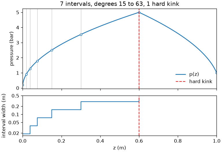
Seven intervals cover the whole metre. Six of them sit in the first 0.3 m, halving
geometrically into the near-vacuum entrance; the entire second stage is a single interval of
degree 63, and the stage boundary is the one hard kink. That is the shape of every useful
D: a lot of local structure in a small part of the fibre, and nothing anywhere else. It is
also why the step cap has to be local. Resolving the same operator over a 4-mode, 2049-point
frequency grid takes about 30 ms and 58 MB.
Interval budget and unresolved tables#
A pathological measured profile can defeat any piecewise polynomial. The builder stops
splitting once the interval budget would be exceeded and flags the remaining intervals as
unresolved. build_phi retries with a looser tolerance, as described below. If the budget
is still exhausted at the maximum tolerance, it returns the unresolved table and logs a
warning that its accuracy is not stated. There is no automatic per-substep quadrature
fallback. Every build also logs its interval count, degrees and width distribution at
DEBUG.
Requirements that are not negotiable#
Each of these has a measured cost when broken, and each is enforced by a test.
Inset the endpoint samples by one ulp of the interval’s own scale. A profile written
z >= z_stagereturns the post-jump value atz_stage, so the interval that ends there otherwise samples the wrong side of its own discontinuity; the search reads that one contaminated sample as unresolvable structure and bisects toward the breakpoint until it hits the width floor. Measured: 21 intervals and an error of 1.5e-8 without the inset, 1 interval and 1.1e-13 with it.Derive the minimum interval width once, from the whole span. Recomputed per call, an already tiny segment recurses several further decades and exhausts the budget without getting any closer to resolving anything.
Track hard kinks apart from split edges, and cap the step by the local interval width rather than the global minimum.
Compute \(n_\text{eff} - 1\) directly, never as \((1 + x) - 1\): the round trip through unity caps the coefficient tail at 1e-12 instead of 2e-16, and the adaptive search can then never reach
tol.Apply any clamping of \(\alpha\) to
Dbefore integration, not to the accumulated exponent afterwards.Supply \(\beta_1\) analytically. A finite-differenced \(\beta_1\) has a relative roughness of about 5e-8 that is independent of the differencing step, so it is an evaluation floor rather than a truncation error, and it caps the whole table at 1e-8.
The table#
Everything above describes the representation. What
solprop.translate.linop.build_phi() actually hands a backend is section 3 of the
kernel contract: a
solprop.translate.linop.LinearOperator, holding the interval edges, the Chebyshev
coefficients of \(\Phi\) over (n_batch_or_1, n_modes, n_pol, n_omega), the degree used on
each interval, the hard kinks steps must land on, and the frame quantities as scalar
tables for the record. Every array is read-only and C-contiguous; nothing else about the
mode, the gas or the frame survives the crossing.
What is tabulated, and over what#
The paths handed to the adaptive builder are the mode’s own core_radius and density
ZProfiles, so their declared breakpoints — the stages of a fill,
the corners of a taper — are the mandatory edges, and the smooth part of their variation is
what drives the split. The array-valued function resolved on the union of those edges is
solprop.linear.dispersion_operator() itself, with the loss policy and the spectral
absorber rate already folded in: the collar is integrated with the dispersion and costs
nothing per step, and a clamp is applied to D and never to the accumulated
exponent.
The frame quantities are tabulated with the same mandatory edges. That is not decoration. Told about the end of a fill, \(\beta_1(z)\) needs three intervals and is good to 7e-15; left to find it, the search bisects toward it until it hits the width floor, spends nineteen intervals, and still leaves a relative error of 1e-11 at the kink itself — a hundred times its own tolerance.
The margin#
The table covers \([0,\ z_\text{max}(1 + \text{margin})]\) with a default margin of five per
cent, because the last step may land exactly on
\(z_\text{max}\) and the noise phase is asked for there, so evaluation at the end must not
fall off the domain. Outside its own span every profile in solprop.profiles holds
its end value, so the margin is a continuation of the fibre rather than an extrapolation of
it, and it costs one interval.
The constant fast path#
A mode set that reports z_constant — a dispersion-specified fibre, a static gas fill —
skips the adaptive build entirely. \(\Phi(z) = Dz\) is a polynomial of degree one, so
solprop.translate.linop.constant_phi() writes a single interval exactly, and the
operator itself is kept alongside it. That second part matters:
solprop.translate.linop.delta_phi() then returns \(D(z_2 - z_1)\) to the last bit
rather than the difference of two Clenshaw sums, so the linear flow of a constant operator
is bitwise reproducible over any pair of positions, which is the property the reference
backend’s linear-only test rests on.
The tolerance is measured, not assumed#
The number asked for is not always the number used. The frame subtracts
\(\beta_0 + \beta_1(\omega - \omega_0)\) from a \(\beta\) that reaches \(8\times10^{7}\
\mathrm{m^{-1}}\) at the top of a wide field grid’s active band, leaving a residual of a few
thousand: about eight digits of cancellation, so one evaluation of D carries an absolute
round-off of order \(10^{-7}\) and a relative one of order \(10^{-11}\). No interpolant can
resolve a function below the noise of its own evaluation, and an adaptive search that is
asked to will bisect until it runs out of budget.
So build_phi measures that floor before it builds — a second difference over a spacing
\(10^{-9}\) of the span, at which the smooth part contributes fifteen orders less than the
noise — and raises the tolerance to a hundred times it. On the RDW gradient capillary
(1.5 m of helium falling from 5 bar to 0.1 bar, 90 nm to 4 µm, 2049 frequency bins) a
build at the nominal 1e-12 exhausts its interval budget after 18.6 s and 1.1 GB; at the
measured tolerance it takes 5 intervals, 0.24 s and 10.3 MB.
The floor is measured in the acceptance test’s own norm, per element against that
element’s own value with the same comparison-scale floor. Measured against the global
envelope instead, the two would not be comparable at all: a problem whose elements span
orders reports a floor set by the largest of them, the tolerance stays far below what the
smallest can be resolved to, the interval budget is exhausted, and the whole search is
paid a second time at a looser tolerance. The spectral collar makes that ordinary rather
than exotic, because its rate is the largest thing in D out of band. On the four-mode
RDW capillary with its absorber:
length |
floor, global norm |
floor, per element |
first build, global |
first build, per element |
|---|---|---|---|---|
1 mm |
1.5e-13 |
2.3e-7 |
415.9 s |
1.09 s |
5 cm |
6.9e-12 |
2.3e-7 |
2.09 s |
1.07 s |
1.5 m |
1.7e-11 |
2.3e-7 |
1.77 s |
1.07 s |
Measuring per element also halves the table, from 181.6 MB to 85.0 MB, and its agreement
with quad_vec is \(5.5\times10^{-11}\) rather than \(2.5\times10^{-12}\) — still an order
inside the \(10^{-10}\) bound, which is itself a decade below the operator’s own noise. The
factor of a hundred above the floor is a safety margin: a measured constant, not a derived
one.
If the budget is exhausted anyway — a pathological measured profile — the tolerance is relaxed by decades up to 1e-7 and the build repeated, each relaxation logged as a warning, before the unresolved table is returned with the warning described above.
Verifying the table#
solprop.translate.linop.verify_phi() is the acceptance test of
the stepper notes, §4 step 3, made a function: \(\Phi(z_2) - \Phi(z_1)\)
against scipy.integrate.quad_vec of D over the same interval, bin by bin, at a handful
of position pairs. The quadrature is the oracle and costs far more than the table, so
build_phi runs it only when debug logging is on, and reports the worst deviation in the
same line as the interval count and the table’s size. On the RDW capillary it is
\(3.7\times10^{-12}\) relative over twenty random pairs — as close to the operator as the
operator is to itself.
The expansion in the parameters#
Everything above resolves D in z. For a mode whose z dependence runs entirely
through scalar paths it declares — a Marcatili mode’s core radius \(a(z)\) and number
density \(\rho(z)\), which
solprop.modes.protocol.ParameterisedMode is the statement of — that is
resolving the wrong variable. D is a function of those parameters,
and the two dependences are nothing alike. D is analytic in the parameters: the gas
susceptibility enters as \(\chi = \gamma\rho\), the waveguide term as \(u^2/(ka)^2\), and the
full model wraps both in a square root that is holomorphic wherever the mode exists. It is
\(\rho(z)\) that is hard — the square-root cusp of a near-vacuum entrance, the stage
boundaries of a fill, the corners of a taper — and \(\rho(z)\) is a scalar.
A mixture keeps this shape when its species follow one total-pressure path: the mode
then declares core_radius and pressure, the composition is folded into an effective
per-particle susceptibility, and the same two-parameter expansion serves. Only
independent per-species density profiles, one density:<label> path each, exceed the
two parameters; those fall to the table of the previous section, which every CPU
backend evaluates (the native backend’s GPU builds refuse it by label).
So D is expanded once over the range each path spans, and \(\Phi\) is that expansion
against scalar integrals along z:
with \(\hat p\) the affine map of the path’s range onto \([-1, 1]\). The only approximation is the truncation in the parameters, because the \(I_{jk}\) are built by the same adaptive machinery on the same declared edges and integrated exactly in the same Chebyshev basis. The hard structure has not gone anywhere; it has moved from arrays of the state’s size into scalar tables of 8 bytes per term per coefficient.
What it costs#
The parameter search is the one-dimensional search of the previous sections applied to each
parameter axis in turn on a tensor grid of Chebyshev–Lobatto points, with the same tail test
and the same noise trim — solprop.translate.expansion.build_expansion(). There is no
splitting in a parameter: one global box per parameter, and a quantity that needs more is
not analytic there and takes the z table instead.
Measured, one mode on the RDW gradient capillary (2049 bins):
z table |
expansion |
|
|---|---|---|
size |
5 intervals of degree 65, 10.3 MB |
9 terms, 0.31 MB |
build |
0.24 s |
0.011 s |
|
0.51 ms |
0.089 ms |
against |
3.7e-12 |
4.8e-12 |
and at the size of a large multimode run — six modes and 16 385 bins on a 1.5 m hydrogen gradient:
z table |
expansion |
|
|---|---|---|
\(\Phi\) |
8 intervals of degree 65, 792.0 MB, 3.53 s |
33 terms, 49.7 MB, 0.88 s |
prefactor |
11 intervals of degree 45, 759.0 MB, 3.11 s |
10 terms, 15.1 MB, 0.25 s |
|
17.8 ms |
1.20 ms |
|
6.16 ms |
0.34 ms |
The two together fall from 1.55 GB to 64.8 MB, and the increments agree to \(5.0\times10^{-9}\) against a tolerance of \(5.4\times10^{-7}\) — the round-off floor of that operator times the safety factor, which is what two independent interpolants of the same noisy function may differ by.
A taper is the one case where the tensor product costs something: expanding in \(a\) needs degree 16 where \(\rho\) needs 8, and a fibre where both vary carries their product, 153 terms and 1.58 MB against the z table’s 4 intervals of degree 65 and 2.07 MB. It is still smaller, and still exact to the same truncation, but the margin is a quarter rather than a factor of fifty.
The logarithmic term on the box#
The expansion carries \(-\tfrac12\ln w\) as well, as an endpoint block beside the
integral one, resolved on the same parameter box
(solprop.translate.expansion.append_endpoint_expansion()). Its tolerance is eight
times the round-off floor of \(\ln w\), and that floor is measured on the box
(solprop.translate.expansion.parameter_roundoff_floor()) as well as along the path,
because the tail test does not look where the path goes. It measures each axis per
element, the samples on the other axis being separate elements, and the box has corners
the path never visits. A taper beside a gradient is the case: the path pairs the high
density with the wide bore, but the box also holds the low-density, wide-bore corner,
where the long-wavelength bins sit near the crossing of \(\operatorname{Re}n_{\rm eff}=1\)
and \(\ln w\) is a few \(10^{-6}\). The rounding of \(\ln w\) is absolute, about one unit in
\(w \approx 1\), so it is a larger relative floor there than anywhere along z. Measured
on a 100 to 80 µm argon taper at 5 to 0.2 bar, the floor is \(1.2\times10^{-12}\) along
the path and \(2.0\times10^{-11}\) on the box. The radius axis’s tail stalls at 1 to
\(2\times10^{-11}\) from degree 16 to 64, so with the tolerance taken from the path’s floor
no degree could meet it and the translation would fail. The box’s floor only ever raises
the tolerance: it changes an expansion that resolves at the path’s floor only if the
looser tolerance accepts an earlier degree, and none of the cases measured does.
Measured against direct samples, that taper’s \(\ln w\) term agrees to \(1.2\times10^{-15}\),
where the declared bound is \(2\times10^{-13}\).
When it is refused#
The expansion is exact only to the truncation of an analytic function of the parameters,
so solprop.translate.expansion.build_expansion() returns nothing — and the caller
builds the z table — whenever:
the mode set does not declare its parameters (a mode beside a capillary one, so there is no shared parameter space; a
solprop.nonlinear.gnlse.SpecifiedModedeclares its effective area and is the case below rather than this one);the modes declare different paths, or paths that disagree in value, so each mode has its own operator rather than one shared with the others. The check is by value at probe positions rather than by identity, because each mode derives its own density object from its own pressure argument;
a mode’s declared parameters are not the whole of its z dependence, which it says by reporting
parameters_own_z = False. Freezing them would silently drop the rest: asolprop.nonlinear.gnlse.SpecifiedModewhose dispersion follows a declared path still declares its effective area, and that area is still its kinks, but it is not everything that moves;an axis is still unresolved at the degree ceiling. That is what a kink in a parameter looks like: the loss clamp of
solprop.linear.LossPolicycrossing its limit partway along the range, the evanescent index floor of a capillary binding partway along it, a measured profile with structure the model does not have.
Which representation was built, and why the other was not, is in the debug log and in
linear.phi_representation.