Radial nodes for expensive responses

This chapter is for single-mode capillary runs where the nonlinear response is so expensive that the number of transverse nodes sets the cost, such as the optional TDSE response and any all-electron atomic model after it. Each node is one atom per call. The chapter says why the radial integral of one HE₁₁ mode is an integral over the field scale, what the effective-area (mode-averaged) model is in those terms and what it gets wrong for ionisation, how the field-scale rules compare with the default, and how to choose. The rules and their qualification are described in SEP 19, which also records the evidence.

The radial integral is an integral over the field scale

For one HE₁₁ mode in a gas that is uniform across the core, the field at radius \(r\) is the axial waveform scaled by \(\eta = J_0(u_{01} r/a)\), with \(u_{01}\) the first zero of \(J_0\). A node’s response depends on \(r\) only through \(\eta\), so the projected source is

\[ S(t) = \int_0^1 F[\eta A](t)\, d\mu(\eta), \qquad d\mu = J_0(u_{01}\xi)\,\xi\,d\xi , \]

one atom per intensity. The linear and Kerr terms are \(\eta\) and \(\eta^3\), so a Gauss rule in \(\eta\) for the measure \(\mu\) integrates both exactly from two nodes, and every error it makes is in the beyond-cubic part: ionisation, the plasma current, the non-perturbative atomic response. Pressure gradients change only the density, and a radius that varies along \(z\) leaves the rule in \(r/a\) unchanged.

The effective-area model is the one-node rule

The mode-averaged model evaluates one response at the effective-area intensity \(P/A_\text{eff}\). In the field scale that is one node at \(\eta_e^2 = M_3/M_1\), with \(M_k = \int\eta^k d\mu\), weighted so that the Kerr term is exact; the linear term is then exact too. For HE₁₁, \(\eta_e = 0.752\): the one atom sees 57% of the axial intensity.

That is why it does badly for ionisation-driven sources. On the SEP 12 helium parent (800 nm, 1 mJ, 6 fs, peak ionised fraction about \(1.6\times10^{-3}\)) it gets the source at the launch plane 85% wrong, and over the run it is 30% off in the generated 120–200 nm energy and up to 16% off in peak power. radial_rule="field_scale", n_r=1 is exactly this model on the resolved route, so it serves as a baseline beside the others – including for a TDSE response, which the mode-averaged route does not take.

How the rules compare

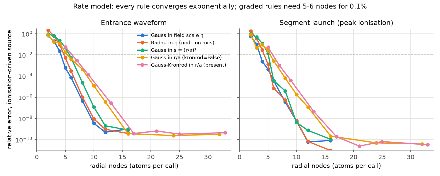
The rate model (PPT ionisation and Kerr) on the SEP 12 waveforms: every rule converges exponentially, and the rules in the field scale need five or six nodes for 0.1%.

The TDSE is different: its current is smooth but oscillates along \(\eta^2\), by about 2% per atom with a period of about 0.15, so a rule must resolve that structure and not only the onset of ionisation. A 157-atom SAE scan of the SEP 12 launch waveform resolves it:

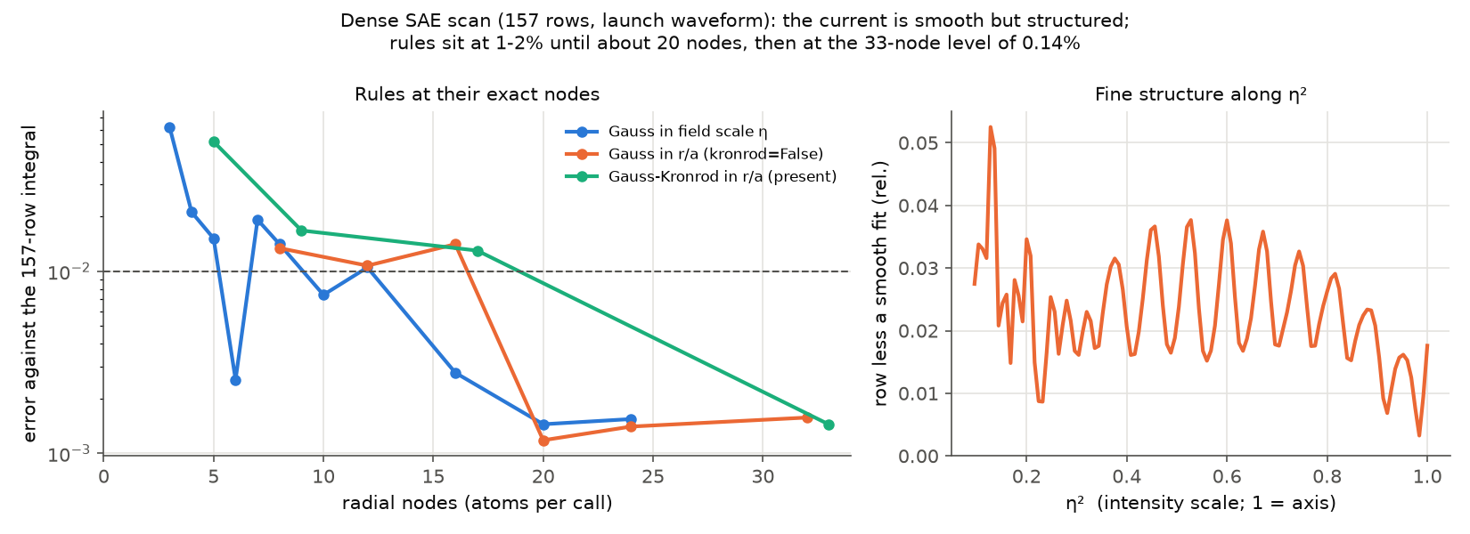
The dense SAE scan. Left: rules at their exact nodes against the 157-atom integral; below about 15 nodes the error is 0.5–2% and depends on where the nodes fall. Right: the per-atom structure the rules have to integrate.

Rule	Nodes	Source error, TDSE scan	120–200 nm field, propagated
Gauss–Kronrod in \(r/a\) (default)	33	0.14%	\(3\times10^{-8}\)
Gauss in \(r/a\)	20	0.12%	≤ 0.02%
Gauss in the field scale	16	0.28%	≤ 0.02%
Gauss in the field scale	8	1.4%	0.1–1.1%
Gauss in the field scale	5	1.5%	0.4–2.0%
Gauss–Radau in the field scale	5	0.38%	–
Gauss in the field scale	4	2.1%	2.2–3.6%
Effective area (one node)	1	–	150%

The propagated column is the rate-model parent run with a calibrated stand-in for the TDSE structure, over four phases of it: it shows how a source error carries through a run, not what a TDSE run gives. In this comparison, a 1–2% source error gives a comparable error in the generated ultraviolet and about ten times less in the field and the peak power. This is not a general bound on error accumulation. Placement matters below about 15 nodes in this study: five Radau nodes happen to land well on this waveform and six do not, so plan on the worst case of a size, not on its luckiest.

These numbers are one waveform and one SAE setup. A stronger field probably puts more periods of structure into \(\eta^2\), and an all-electron model needs its own study: the rule construction carries over, the node counts do not.

Choosing

The following are starting points from the study above, not accuracy guarantees for a different waveform or atomic model. Converge the observable you need.

Goal	Setting
The default, with the quadrature alarm	radial_rule="gauss_kronrod", n_r=32 (33 nodes)
Sub-percent, no special rule	radial_rule="gauss", n_r=20
Sub-percent, fewer atoms	radial_rule="field_scale", n_r=16
Percent level, for exploration and all-electron models	radial_rule="field_scale", n_r=5 to 8
As above, with an atom on the axis	radial_rule="field_scale_radau", n_r=5 to 8
The effective-area comparison	radial_rule="field_scale", n_r=1
Not for quantitative ionisation	fewer than four nodes

A rule is chosen where the capillary is built:

import warnings

from solprop.driver import Simulation
from solprop.exceptions import MaterialRangeWarning
from solprop.stats import StatsSpec

with warnings.catch_warnings():
    warnings.simplefilter("ignore", MaterialRangeWarning)
    simulation = Simulation.from_capillary(
        125e-6,
        0.1,
        "Ar",
        1.0,
        lambda0=800e-9,
        fwhm=10e-15,
        energy=1e-4,
        plasma=True,
        modes=1,
        trange=100e-15,
        wavelength_limits=(300e-9, 2e-6),
        radial_rule="field_scale_radau",
        n_r=5,
        stats=StatsSpec(
            names=("energy", "electron_density", "on_axis_electron_density")
        ),
    )
print(simulation.settings.quadrature.n_nodes)  # 5 atoms per call instead of 33

and for an explicitly configured response such as the TDSE, on the rule itself:

from solprop.modes import MarcatiliMode, transverse_quadrature

mode = MarcatiliMode(125e-6, "He", 1.0)
rule = transverse_quadrature([mode], n_r=8, radial_rule="field_scale")
# then Simulation(grid, [mode], [tdse], initial,
#                 settings=replace(tdse_settings, quadrature=rule))
print(rule.n_nodes, rule.has_embedded_rule)

The cost. On a CPU, and for all-electron models, the cost of a call is nearly linear in the node count, so eight nodes cost about a quarter of 33. A GPU running SAE atoms is far from full at 33 rows, so fewer rows save little there (1.2–2.2× on the measured cards); the same budget may be better spent on more rows.

What the rules refuse. The field-scale rules need exactly one Marcatili HE₁₁ mode: several modes, a higher HE₁ₘ mode, or a mode whose radial profile is not \(J_0\) are refused by name, because the field at a node is then no longer one waveform times a scale. They have no embedded coarse rule, so the quadrature alarm is off, as with "gauss". Their area weights integrate the source, not the area: five Gauss nodes’ weights sum to 0.96 of the core, and integrated quantities such as the ionised inventory species_ionisation_energy carry that quadrature error and need their own check. The Radau rule needs at least four nodes; one node is admitted for "field_scale" alone.

The plasma statistics and the axis

electron_density and the peak rates are read at the rule’s nodes – the densest node, and maxima over nodes. With the default rule a node sits near the axis, so they approximate the axial values; they remain sampled maxima. With five Gauss field-scale nodes the innermost sees 92% of the axial intensity, and the reported density can be half the axial one; such a run warns with a SampledPeakWarning. Ask for the on-axis statistics instead: on_axis_electron_density, on_axis_peak_ionisation_rate and their species forms read the field synthesised on the axis, at the cost of one extra row’s rate scan per saved plane – or none with the Radau rule, whose first node is the axis. The TDSE route defines no plasma statistic and never evaluates an atom for one. The definitions are on the statistics page.