Strong-field ionisation

The ionisation rate W(|E|) is the probability per unit time that one atom loses its outermost electron in a field of amplitude |E|. It is the input to the plasma response: the fraction ionised is 1 − exp(−∫W dt), the free electrons shift the refractive index downwards, and the field pays one ionisation potential for each electron it frees. In a hollow capillary filled with a noble gas it can arrest self-compression, blue-shift the driving pulse and change the phase matching of a resonant dispersive wave. Its importance depends on the ionised fraction and on the competing dispersion and nonlinear responses.

Choose the ionisation rate and the optical current model separately. Optmat supplies the built-in rate models; solprop couples the resulting population and currents to propagation. A converged rate table only controls interpolation error, not the uncertainty of the atomic or molecular rate itself.

The radial filament lesson shows how to read plasma and intensity together. This chapter covers rate selection, data, thresholds and interpolation. Carrier-resolved plasma and envelope plasma give the corresponding current models, energy accounting and limits. Where solprop’s choices differ from Luna.jl’s, the differences are listed in Noteworthy differences from Luna.

Which rate a run uses

prop_capillary, prop_waveguide and their Simulation constructors take each species’ rate from optmat when plasma is True, or left unset on a field grid: the recommended rate model of the gas at the run’s carrier (rates from optmat). Air (gas="air") is ionised through the nitrogen and oxygen populations of the mixture, each with its own rate (below).

On an envelope grid (envelope=True) plasma is off unless plasma=True or a rate is given, and the rate is then cycle-averaged by the response itself (envelope plasma sources). plasma=False turns it off; a rate object is used as given; a mapping from mixture label to switch or rate selects per component, and omitted labels are off. solprop.nonlinear.mixtures.responses_for() applies the same per-species defaults but has plasma=False by default, and the free-space routes take explicit response objects: naming the gas alone does not enable ionisation there.

Rates from optmat

optmat curates strong-field rate models for every gas solprop ships, checked against all-electron static rates, a time-dependent calculation and measured yields. solprop takes them, and keeps no formula of its own (SEP 3). The free-space and planar routes, whose rates are the caller’s, bind an OptmatRate’s energy per event to the input’s peak field as the capillary route does.

OptmatRate adapts one optmat rate model to the rate protocol: an atom’s through optmat’s ionisation_rate_model, a molecule’s through molecular_rate_model (each refuses the other’s species), or a model object taken as it is:

from optmat.gas.ionisation_rates import ionisation_rate_model

from solprop.nonlinear.optmat_rates import OptmatRate

argon = OptmatRate("Ar", 800e-9)  # optmat's recommended rate
literature = OptmatRate("N2", 800e-9, model="moadk_zhao_2010")
doubled = OptmatRate(ionisation_rate_model("Ar", 800e-9).with_parameters(electrons=2.0))

prop_capillary(...) with plasma=True builds the first of these for each species; MaterialSelection(ionisation="ppt_ilkov") names a literature form instead, and MaterialSelection(ionisation=model) takes an optmat model object. The carrier is the selection’s carrier_wavelength, or the run’s lambda0. A custom species (a name solprop does not ship, or a built-in name with its own ionisation data) has no default rate and is refused by name: its rate is given explicitly, plasma={label: OptmatRate(IonisationRateModel.from_parameters(...))} with optmat’s explicit-parameter constructor, or a rate of the caller’s own (below).

The models. All of optmat’s rates are for linear polarisation, take the field in V/m and return s⁻¹. At optmat 0.8.0 (unchanged since 0.4.0) the recommended models are, with the adapter’s values at 800 nm (the threshold below which the rate is exactly zero, the maximum field above which it is held, and the energy per event in the weak-field limit):

species	model	effective electrons	uncertainty factor	threshold (V/m)	maximum field (V/m)	energy per event (eV)
He	short-range PPT with the frequency-dependent Coulomb factor and Tong and Lin’s correction	1.47	1.3	1.3 × 10⁹	2.1 × 10¹¹	24.59
Ne, Ar	as He, with the ion’s two fine-structure channels	1	1.5	7.4 × 10⁸, 1.2 × 10⁸	1.6 × 10¹¹, 8.6 × 10¹⁰	21.56, 15.76
Kr, Xe	as Ne, with Tong and Lin’s suggested α = 9	1.35, 1.5	2, 3	5.0 × 10⁷, 1.5 × 10⁷	6.8 × 10¹⁰, 5.1 × 10¹⁰	14.00, 12.13
H₂, D₂	molecular model, orientation-averaged structure factors	2	1.5 / 2	7.2 × 10⁷	7.2 × 10¹⁰	16.06 (vertical)
N₂	molecular model	2	1.5	9.6 × 10⁷	7.2 × 10¹⁰	15.58 (vertical)
O₂, N₂O	molecular model	2 / 4	2 / 3	1.5 × 10⁷, 1.9 × 10⁷	5.2 × 10¹⁰, 4.9 × 10¹⁰	12.31, 12.89 (vertical)
CH₄	molecular model, Zhao et al.’s 2011 structure	6	2	4.7 × 10⁷	6.2 × 10¹⁰	14.40 (vertical)
SF₆	molecular model, an untested prediction (status untested)	6	10	8.1 × 10⁷	7.3 × 10¹⁰	15.69 (vertical)

The effective electron number is optmat’s: helium’s 1.47 comes from its two-electron comparison, and an occupancy of two on top of it would double an already correct low-field helium rate; krypton’s 1.35 and xenon’s 1.5 come from Wallace et al.’s measured yields, as no all-electron rate of either atom exists. The atomic models carry no Stark shift or dipole factor, which would count twice what the fitted structure already contains. The uncertainty factor describes the model — the factor within which optmat expects the rate to be right between 10⁻⁶ of saturation and saturation — and is recorded in the run’s manifest; it is not a software tolerance. The named literature forms (ppt_ilkov, ppt_larochelle, ppt_popruzhenko for an atom; moadk_zhao_2010, moadk_tong_2002, moadk_zhao_2017, ppt_talebpour, ppt_talebpour_ilkov, adk_hydrogenic for a molecule) are status comparison, and stay selectable.

The threshold. The adapter’s rate is exactly zero below the field at which optmat’s instantaneous rate falls under a declared negligible rate, NEGLIGIBLE_RATE (10⁻³⁰ s⁻¹: one atom in 10⁴² over a picosecond), found by bisection in the logarithm of the field. Above it the rate is optmat’s, capped at MAX_RATE, and tabulated by the same table as every other rate.

The maximum field. Each model declares the largest field its static correction was fitted to: twice the barrier-suppression field with Tong and Lin’s correction (an atom), 4.5 times with Zhang’s, 1.5 times for the molecules. Above it optmat’s instantaneous rate leaves its fit: it turns over a few per cent above the maximum field (4–7 % for Ar, Kr and Xe, 16–19 % for N₂ and He), is erratic beyond (argon’s spikes to 2600 times its value at the maximum field at 1.6 times that field) and falls towards zero within a decade, and a rate table, which by default reaches thirty times the input’s peak, would extend there. The adapter therefore holds the rate at its value at the maximum field above it, as a table holds its last knot, and the table stops there. Holding is the least bad of the choices: at that rate a population is depleted within a femtosecond, so the held value already ionises everything it reaches. optmat warns at every evaluation above the maximum field; a direct evaluation there is recorded in the run’s manifest (ranges) instead of warned, and a table, which ends at the maximum field, records nothing. A run warns once when the input’s own peak field exceeds the maximum, and whether the run reached it is the post-run diagnostic’s to say (below): it warns once when a population’s recorded peak rate reached the held value. The hold leaves a corner in the rate at the maximum field, which a transverse quadrature resolves only slowly, so a run that goes there also meets the backend’s quadrature alarm; it is outside the model’s fitted range either way, and how to continue a rate beyond it is an open question.

The energy per event. The plasma loss pays the energy the rate’s own exponent uses: optmat’s rate-weighted energy \(\bar I(E) = L(E)/W(E)\), with \(L = \sum_c I_c W_c\) over the channels the model sums. For the molecules that is the vertical ionisation energy the rate uses, not the adiabatic one. For the noble gases it moves with the field between the two fine-structure channels — for argon at 800 nm from about 15.78 eV near the threshold to 15.82 eV at the maximum field, for xenon, whose channels are 1.31 eV apart, by 2.4 % — and solprop’s kernel carries one energy per population. The loss therefore takes a constant, \(\bar I(E_\text{ref})\) at a reference field: the input’s peak field amplitude, the one that sets the default range of the rate table (default_field_range), which the capillary and waveguide drivers bind, clipped to the tabulated fields above the threshold. An explicit rate keeps its own reference_field; a rate without one takes the weak-field limit, the lowest channel’s energy. The rate records the bound of that constant, \(\max|\bar I(E)/\bar I(E_\text{ref}) - 1|\) over the tabulated fields at which the rate is not negligible (energy_bound, over energy_span). A one-channel model, every molecular one among them, is exact. In the tunnelling exponent a small change of threshold is not a small change of rate, so the constant replaces only the loss, never the rate’s own energies. A plasma response given an OptmatRate stores its species with that energy as its potential (bind_rate_energy()), so the field formulation’s loss term, the envelope’s loss current and the species statistics all pay it.

Polarisation. The rates are for a linearly polarised field. An elliptical or circular run stays admitted, as before, on the quasi-static average of the instantaneous rate around the polarisation ellipse, and the manifest records the approximation. A run whose input is not linearly polarised at its peak, at a Keldysh parameter above one there, warns once: there elliptic and orbital-resolved theories depart from that average. The check runs where the input’s polarisation is known: on a free-space route from the pulse’s Jones vector (a spectrum given as an array is taken as linear), and in Simulation.with_input from the new input’s field over the axis and the nodes. A capillary or waveguide constructor launches one scalar pulse in one mode, which is linear at every node. with_input keeps the reference field and the table range of the run it derives from, and checks the new input against each rate’s maximum field as well. On an envelope grid the cycle average at linear polarisation is checked against optmat’s own cycle_averaged_rate, which its “consistent” averaging makes agree with the cycle average of the instantaneous rate to 3 % up to the barrier-suppression field; the agreement measured is within 2 %.

After the run. peak_field_report() turns each population’s recorded peak rate (species_peak_ionisation_rate, at the save planes) back into the largest field it saw — self-compression can raise it above the input’s — through the rate the statistic records: the table’s rate of |E| on a field grid, and on an envelope grid the run’s own cycle average of its table at linear polarisation (linear_cycle_average() is the same average, and linear_cycle_averages() evaluates it at many amplitudes from one call of the rate, to the adaptive quadrature’s \(2\times10^{-10}\)), not optmat’s cycle_averaged_rate, which departs from it above the barrier-suppression field. It compares the field with the model’s maximum field, and \(\bar I\) there with the constant the loss paid. Simulation.run reports it, and Simulation.material_manifest() then carries it (peak_fields); the file’s record, written before the run, carries the inputs to it — the maximum field, the reference field, the constant and its bound (policies["ionisation"]) — and the peak rates. The run writes the report itself into its output when it closes, as the post-run annotation "material_peak_fields", outside the configuration hash (output), so a file read back later carries the result beside its inputs.

Carrier. optmat compared its rates with references down to 350 nm, and warns below; solprop translates that warning once per run, and records it.

How far to trust them. Curated data do not make an approximate rate theory accurate everywhere, and optmat reports its own discrepancies. Helium is within about 20 % of all-electron static and laser-field rates. For argon, krypton and xenon optmat shows both absolute-yield comparisons: the recommended rates reproduce the 5.5 fs calibration-standard yields of Wallace et al. (2016) within that experiment’s calibration, and are 1.7 to 8 times above the 42 fs absolute yields of Wahlstrand et al. (2018). That disagreement is unresolved upstream; solprop neither rescales the rate nor picks a winner, and the uncertainty factor is the summary. SF₆’s rate has no reference at all, which is why it is untested, warns once per run, and carries a factor of 10.

A rate of your own

Any object that satisfies IonisationRate can be given as plasma= (per label for a mixture) or to a PlasmaResponse. The protocol asks for:

• __call__(field_amplitude): the rate per atom or molecule in s⁻¹ for a field amplitude in V/m, vectorised and even in the sign of the field;

• threshold: the field in V/m below which the rate is exactly zero;

• maximum: the ceiling in s⁻¹ at which the rate is clipped, MAX_RATE unless there is a reason for another;

• citation: one line naming the model and the options in force;

• parameters: every setting that changes the rate, as name-sorted (name, value) pairs, from which the table cache key is built.

Three optional attributes complete it. convention declares the optical-cycle convention (rate_convention()): "instantaneous-isotropic" for a rate of the instantaneous |E|, which the envelope route requires, or "cycle-averaged". gas (or species_identity with ionisation_potential) names the species, which the response checks against its own (rate_species()). plasma_energy, beside species_identity, declares the energy per event the loss pays (rate_energy()); without it the response pays the species’ ionisation potential. A callable with none of this, EvaluableRate, is enough for ionisation_fraction() and for a response given a tabulated RateTable, but a kernel needs the threshold and ceiling to build its table.

A rate from explicit parameters is better written as an optmat model, OptmatRate(IonisationRateModel.from_parameters(...)), which then carries optmat’s threshold, maximum field, energy per event and record as a built-in rate does. A rate known only at samples (from measured yields, or a time-dependent calculation) is a rate of your own whose __call__ interpolates them, which build_rate_table() then tabulates like any other.

Two regimes and one parameter

A bound electron can absorb many photons at once and leave over the barrier, or it can tunnel through the barrier the field bends. Which of the two describes a given field is characterised by the Keldysh parameter, the characteristic tunnelling time divided by the optical timescale \(1/\omega\),

\[ \gamma = \frac{\omega \sqrt{2 I_p}}{E} \quad \text{(atomic units)}, \]

evaluated by solprop.nonlinear.ionisation.keldysh(). Ionisation is multiphoton for γ ≫ 1 and quasistatic tunnelling for γ ≪ 1; in a 800 nm field, argon crosses γ = 1 at about 3 × 10¹⁰ V/m, which is where a self-compressing pulse in a capillary spends most of its peak.

Above the barrier-suppression field

\[ E_b = \frac{I_p^2}{4 Z} \quad \text{(atomic units)}, \]

solprop.nonlinear.ionisation.barrier_suppression_field(), the barrier is pulled below the level altogether and there is nothing left to tunnel through. For helium at 1.05 × 10¹¹ V/m, for xenon at 2.6 × 10¹⁰.

Thresholds, ceilings and why both exist

Every rate is exactly zero below a declared threshold field. This is not an optimisation: the plasma loss term is Ip W (1−f)/E, which divides by the field, and it is finite only because the rate vanishes identically where the field is small. An optmat rate’s threshold is the field at which its rate falls to NEGLIGIBLE_RATE (above), so nothing physical is discarded.

Every rate is clipped at a declared maximum, one ionisation per atomic unit of time (MAX_RATE, 4.1 × 10¹⁶ s⁻¹) by default. A rate at or beyond that would free the electron in less than an orbit, which is where the quasistatic expansion has stopped meaning anything; the clip is what stops a diverged coarse step turning an overflow into a NaN that then poisons the whole convergence ladder (stepper design, §10).

Tables

Evaluating an optmat rate model directly costs microseconds per sample, vectorised over a whole column. A propagation evaluates the rate once per sample of the fine time grid, on every column, at every stage, so it uses a precomputed table: solprop.translate.ionisation.RateTable, built by solprop.translate.ionisation.build_rate_table(), which brings that to about 10 ns in NumPy; the compiled backends evaluate the same table inside their kernels. The table controls interpolation accuracy and behaviour outside its sampled interval. Its tolerance is separate from the optical stepper tolerance and the rate model’s physical uncertainty.

• Knots are uniform in log E, so locating one is arithmetic rather than a search, and a single table spans two to four decades. log W is nearly linear in log E at the low-field turn-on and flattens at high field, which is where the samples are needed.

• The knot count is converged, not fixed: it doubles until the interpolant is within rtol (10⁻⁶ by default) of direct evaluation at three probe points per interval, measured as a difference of logarithms so that it stays meaningful where the rate is 10⁻³⁰⁰. A few hundred knots suffice for a smooth rate.

• Both ends are clipped: exactly zero below field_min, and held at the last value above field_max rather than extrapolated, because a cubic in log W continued past its last knot is precisely how a diverged step becomes an infinity, and raising instead would abort a propagation in the middle.

• The cache key is deterministic: it is built from the rate’s own parameters, sorted by name, so no ordering of keyword arguments can give two keys for one rate. The solprop.translate.ionisation.RateTable.key digest is stable across processes.

import warnings

import numpy as np
import matplotlib.pyplot as plt

from solprop.nonlinear.ionisation import barrier_suppression_field
from solprop.nonlinear.optmat_rates import OptmatRate
from solprop.physdata import Gas, ionisation_potential

gases = [Gas.He, Gas.Ne, Gas.Ar, Gas.Kr, Gas.Xe]

fig, ax = plt.subplots(figsize=(6.0, 3.8))
for index, gas in enumerate(gases):
    rate = OptmatRate(gas, 800e-9)
    barrier = barrier_suppression_field(ionisation_potential(gas), 1.0)
    field = np.geomspace(0.1 * barrier, rate.maximum_field, 400)
    with warnings.catch_warnings():
        warnings.simplefilter("ignore")
        values = rate(field)
        at_barrier = float(rate(barrier))
    ax.loglog(field, values, color=f"C{index}", label=gas.value)
    ax.plot(barrier, at_barrier, "o", color=f"C{index}")
ax.set_ylim(1e2, 1e17)
ax.set_xlabel("field amplitude (V/m)")
ax.set_ylabel("ionisation rate (1/s)")
ax.legend(frameon=False, ncols=2, fontsize="small")
fig.tight_layout()

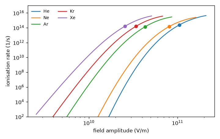
optmat’s recommended rates for the five noble gases at 800 nm, each marked at its barrier-suppression field and drawn up to its maximum field, twice that.

A worked example

from solprop.nonlinear.ionisation import ionisation_fraction
from solprop.nonlinear.optmat_rates import OptmatRate
from solprop.translate.ionisation import build_rate_table
import numpy as np

rate = OptmatRate("Ar", 800e-9)                # optmat's recommended argon rate
table = build_rate_table(rate, (1e9, 1e11))    # converged to 1e-6, log-spaced knots

t = np.linspace(-40e-15, 40e-15, 2049)
field = 4e10 * np.exp(-(t / 10e-15) ** 2)      # 4e10 V/m peak, 17 fs FWHM in field
fraction = ionisation_fraction(table, field, float(t[1] - t[0]))
print(f"{100 * fraction[-1]:.2f} % ionised")   # 44.72 % ionised

Molecules: an orientation-averaged rate

optmat’s molecular models average the rate over an isotropic distribution of molecular orientations (orientation-averaged structure factors). The average is of the rate, before depletion. For frozen orientations,

\[ 1-e^{-\int\langle W\rangle dt} \geq \left\langle1-e^{-\int W(\theta)dt}\right\rangle, \]

so the two agree in the weak-depletion limit and the averaged rate overstates the ionised fraction once depletion matters. Alignment, rotational motion and orientation-selective depletion of the neutrals are not evolved. The rate is instantaneous, not cycle averaged: PlasmaResponse evaluates it on the instantaneous real field, and EnvelopePlasmaResponse performs the optical-cycle average itself.

The plasma is single ionisation: it depletes a molecule once, creates at most one electron and pays one energy per event. Ionisation is also distinct from dissociation: no neutral fragment yield, branching ratio, recombination or ozone production is modelled.

Ionisation in air and other mixtures

Air has no single ionisation potential, and the dispersion-only Gas.Air carries no ionisation data. gas="air" (nitrogen and oxygen) or Mixture.air(...) (with argon) give each species its own plasma channel instead, by default with optmat’s rate of that species (which rate a run uses). A mapping overrides that per label; for example plasma={"N2": OptmatRate("N2", 800e-9, model="moadk_tong_2002"), "O2": True} takes a named literature form for nitrogen and the recommended rate for oxygen, and leaves argon, whose label it omits, without a plasma channel. Each population has its own initial fraction, rate table and exposure scan under the common real field. The five species statistics retain every component, including those without a channel. The density input is the species’ own number density; no oxygen-fraction rescaling of a total-air density is needed. Final ionised inventory includes preionisation; pulse-produced electrons subtract the initial fraction before converting a result into a chemical increment. The initial fraction may be a path along z per population, such as preionisation={"N2": PiecewiseLinear(...), "O2": 0.0}: the fraction ionised before the pulse arrives at each position, read by every backend at every stage, with the steps landing on the path’s kinks (nonlinear.md).

Envelope plasma sources

The dedicated model chapter explains the physical origins, vector derivation, spectral signs, alternative theories and validity limits. This section is the practical API and numerical-policy summary.

Gas-filled capillary and waveguide constructors select this response when envelope=True and plasma=True, or when an instantaneous rate is explicitly supplied as plasma. Leaving plasma unspecified retains the envelope default of no plasma. Per-label rate mappings select independent mixture populations. For example:

from solprop.driver import Simulation

simulation = Simulation.from_capillary(
    125e-6,  # core radius, m
    0.3,  # length, m
    "Ar",
    1.0,  # pressure, bar
    lambda0=800e-9,
    wavelength_limits=(500e-9, 1.2e-6),
    trange=80e-15,
    fwhm=20e-15,
    energy=1e-5,
    envelope=True,
    plasma=True,
    raman=False,
    backend="numpy_ref",
)

Envelope third-harmonic generation cannot be combined with plasma. An ordinary species-free prop_gnlse model has no plasma.

solprop.nonlinear.envelope_plasma.EnvelopePlasmaResponse accepts a physical complex envelope in V/m, with one or two Cartesian components. Modal amplitudes in √W must first be converted with the mode’s normalisation. The response returns separate currents and the population; these currents are combined with ordinary nonlinear polarisation only after their forward transforms.

A saved amplitude needs one step before that normalisation: it is the true-power amplitude \(b=\sqrt w\,a\) (power and intensity), so it must be divided by \(\sqrt{\operatorname{Re}n_{\rm eff}}\) first — solprop.processing.mixtures.get_power_weight() returns that \(w\) for every saved plane — and only then converted to V/m. Skipping the division is not a small error where a rate is concerned: the logarithmic slope of a tunnelling rate against field is about 170 near the peak of a capillary run, so a field wrong by \(10^{-4}\) moves the rate by about 2 %.

Write the real field around a frozen cycle as \(E_\theta=\operatorname{Re}(a e^{-i\theta})\). For an isotropic instantaneous rate \(W(|E|)\), define

\[ \overline W(a)=\frac{1}{2\pi}\int_0^{2\pi}W(|E_\theta|)\,d\theta, \qquad j_L=2I_p\rho s\left\langle \frac{W(|E_\theta|)E_\theta}{|E_\theta|^2}e^{i\theta} \right\rangle. \]

Here \(\rho\) is the initial particle density, \(f\) the ionised fraction and \(s\) the surviving neutral fraction. The population uses the same trapezoidal prefix convention as the field route, with zero exposure at the first sample:

\[ H_0=0,\quad H_j=H_{j-1}+\tfrac{\Delta t}{2}(\overline W_{j-1}+\overline W_j), \quad f=f_0+(1-f_0)[-\operatorname{expm1}(-H)],\quad s=(1-f_0)e^{-H}. \]

Keeping \(s\) directly preserves the remaining ionisation loss even after \(f\) rounds to one. The Drude drive is \(d_D=(e^2/m_e)\rho f a\), in A m⁻² s⁻¹; \(j_L\) is in A m⁻². Cycle work satisfies \(\operatorname{Re}(a^\dagger j_L)/2=I_p\rho s\overline W\). In an intermediate ellipse, the loss current generally has different weights along the two principal axes. A scalar multiplier of \(a\) can reproduce the total work while giving the wrong vector current.

The independent physical oracle integrates the Cartesian cycle adaptively. For propagation, translation compiles the instantaneous magnitude rate into a one-dimensional spline and integrates both ellipse moments using split Gauss–Legendre rules. It compares orders 64 and 128, then 256 and 512 if needed, with a 2e-6 relative budget per moment and a 1e-30 s⁻¹ comparison floor. An unresolved moment raises a convergence error. The rate-table interpolation budget is separate (1e-7 in log rate), and its lower boundary follows the rate model’s threshold. An explicit RateTable retains its own clipping policy.

For example, to inspect a circular-envelope population and source directly:

import numpy as np
from solprop.nonlinear import EnvelopePlasmaResponse
from solprop.nonlinear.optmat_rates import OptmatRate

t = np.linspace(-20e-15, 20e-15, 33)
amplitude = 3e10 * np.exp(-((t / 10e-15) ** 2))
field = np.stack((amplitude, 1j * amplitude))
response = EnvelopePlasmaResponse("Ar", OptmatRate("Ar", 800e-9), preionisation=0.1)
source = response.sources(field, 2.5e25, dt=float(t[1] - t[0]))
assert source.fraction[0] == 0.1
assert source.loss_current.shape == field.shape

The compiled internal-FFT source factors are -1/omega**2 for the Drude drive and -1j/omega for the loss current. omega is the absolute positive optical frequency, not detuning. Both factors are zero outside the active band; DC and negative frequencies are never inverted. In the optics convention the loss factor is +1j/omega. Projection precedes the temporal forward transforms where the geometry permits, and the material-source time collar applies to each stream.

shock=False freezes these two factors and the explicit UPPE numerator at the carrier frequency. Translation warns once and records this approximation in configuration/provenance. The frequency-dependent mode index and active masks remain in force, and the spatial routes’ restriction on shock=False applies.

A rate on this route must be instantaneous: OptmatRate declares convention = "instantaneous-isotropic", and the convention retained by RateTable distinguishes instantaneous and already averaged inputs. A custom magnitude callable must explicitly declare convention = "instantaneous-isotropic"; compilation also requires the threshold, maximum and parameter declarations used by IonisationRate. A rate’s declared chemical species and binding energy must agree with the response.

Saved-plane and periodic population statistics use the same cycle-averaged rate as propagation. The statistics have the same names as on a field grid; peak-rate entries carry "cycle-averaged" in statistic_rate_conventions metadata. Population histories start at the declared preionisation on every evaluation – at a path’s value at that position when the preionisation varies along z. Resume, mixture replacement and fixed-schedule scans recompute those histories from the current field.

This model assumes slow envelope evolution and small depletion within an optical cycle. It uses the same instantaneous rates as the field grid; the cycle integration does not make them nonadiabatic or supply an orbital-resolved elliptic PPT rate. A phase-resolved (Yudin–Ivanov) rate would need a loss-current closure of its own, which is why it is not offered (envelope plasma). Collisions, recombination and sequential charge states are outside this route.

The carrier/envelope gallery comparison shows two complete deterministic runs with the same instantaneous argon rate and plots their populations and fundamental spectra. It is an illustration at one resolution; the numerical accuracy and validity limits are discussed in the envelope plasma chapter.