Free space: beams in bulk media#
This guide is for propagating a beam through a bulk medium — a gas cell, a gas jet, a window, vacuum — rather than along a waveguide: diffraction, self-focusing, filamentation and ionisation, and the spectral broadening that comes with them. A free-space run evolves the electric field itself on a transverse grid, with the exact (non-paraxial) diffraction operator, and it shares everything else with the fibre routes: the time grids, the pulses, the Kerr, plasma and Raman responses, the stepper, the output files and the backends. The derivations — the operator, the field units, the absorbing collar and the critical power — are on the reference page, the free-space model, and what energy and intensity mean in a medium is energy and flux in a medium; this page is how to use it.
Every snippet on this page runs as written, in seconds (the test suite executes them in order), and may build on the ones before it.
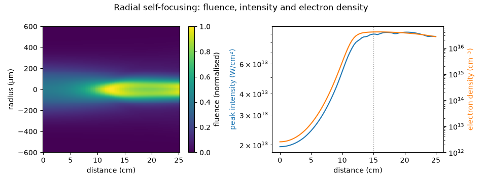
A filament in argon at 1 bar, from the filamentation tutorial: a 0.88 mJ, 30 fs beam at three times the critical power self-focuses, ionises the gas and leaves a channel whose intensity is clamped by the plasma. Left, the fluence along the propagation, mirrored about the axis; right, the peak intensity and the electron density. The run takes seconds.#
Choosing a grid#
Three transverse grids, one entry point each; the spectral columns each evolves and the media each accepts are defined in the free-space model:
grid |
resolves |
use it for |
entry point |
|---|---|---|---|
\(r\), assuming each polarisation component is cylindrically symmetric |
round beams on axis: focusing, self-focusing, a single filament; the cheapest |
|
|
\(x\) and \(y\), a periodic box |
anything without that symmetry: a tilted, astigmatic or elliptical beam, several filaments, beam break-up |
|
|
\(x\) alone; uniform in \(y\) |
a sheet beam, per metre of \(y\) |
|

The radial grid samples at the zeros of \(J_0\), the nodes of the order-zero Hankel transform, so the field vanishes at the grid’s radius \(R\). Its outer tenth is a collar that absorbs whatever reaches it, when the run declares an absorber.#

The Cartesian box is periodic and assumes no symmetry; it costs \(n_x n_y\) columns per time sample, so memory is what limits it.#

The line is the Cartesian grid’s x axis alone: the beam is uniform in y, so energies are in J/m and powers in W/m.#
A planar guide resolved across its width, prop_planar, is the same idea for a beam of
finite height between two plates; it is described with the other guides, in
guided propagation.
A beam in argon#
A beam is a temporal pulse wrapped in a transverse profile,
SpatialPulse; waist is the 1/e² intensity radius, and the
pulse’s energy or peak_power is the whole beam’s physical energy or peak power in the
medium at the launch plane (energy and flux in a medium). The medium is a
SpatialMedium — a gas at a pressure, a glass, or a constant
index; SpatialMedium() is vacuum. The responses are the same objects the fibre routes
use. Here a 100 µm beam at 1.5 times the critical power propagates a centimetre
through argon with the Kerr effect, on an envelope grid, saving ten planes:
import numpy as np

from solprop.boundaries import absorber
from solprop.driver import SimulationSettings, prop_radial
from solprop.grid import EnvelopeGrid, RadialGrid
from solprop.nonlinear.responses import KerrResponse
from solprop.constants import C
from solprop.physdata import chi3, gamma3, refractive_index
from solprop.pulses import GaussianPulse, SpatialPulse
from solprop.spatial import SpatialMedium, critical_power
from solprop.stats import StatsSpec
from solprop.stepper import PIController

length, planes = 1e-2, 10
argon = SpatialMedium("Ar", pressure=1.0)
n0 = float(refractive_index("Ar", 2 * np.pi * C / 800e-9, pressure=1.0))
power = critical_power(800e-9, chi3("Ar", pressure=1.0, wavelength=800e-9), index=n0)
print(f"critical power in argon at 1 bar: {power * 1e-9:.3g} GW")

grid = EnvelopeGrid.from_limits(length, 800e-9, (600e-9, 1.2e-6), 200e-15, thg=False)
space = RadialGrid(radius=400e-6, n_r=64)
beam = SpatialPulse(
    GaussianPulse(wavelength=800e-9, fwhm=30e-15, peak_power=1.5 * power),
    waist=100e-6,
)
settings = SimulationSettings(
    controller=PIController(rtol=1e-6, atol=1e-12),
    save_planes=np.linspace(0, length, planes + 1)[1:],
    dz_init=1e-4,
    dz_max=length / planes,
    stats=StatsSpec(names=("energy", "beam_radius", "peak_intensity")),
    absorber=absorber(grid),
)
run = prop_radial(
    grid,
    space,
    argon,
    [KerrResponse(gamma3("Ar", wavelength=800e-9), thg=False)],
    beam,
    settings=settings,
    progress="none",
)
The statistics are recorded at every saved plane. beam_radius holds two radii of the
fluence: the second moment (index 0), which the wings dominate, and the interpolated
radius at which the fluence falls to 1/e² of its peak (index 1), which follows the core;
peak_intensity is the largest axial flux over the grid:
radius = np.asarray(run["stats/beam_radius"])[..., 1].reshape(-1)
intensity = np.asarray(run["stats/peak_intensity"]).reshape(-1)
for z, w, peak in zip(np.asarray(run["z"]), radius, intensity, strict=True):
    print(f"z = {z * 1e3:4.1f} mm: radius {w * 1e6:5.1f} um, {peak * 1e-4:.3g} W/cm²")
Over a centimetre, a quarter of the beam’s Rayleigh length, the Kerr lens has begun to contract it, and the peak intensity, near 10¹⁴ W/cm², is already where argon starts to ionise. The model page derives the critical power and says what it does and does not predict for a pulse.
The absorber. absorber(grid) makes the outer tenth of the spatial grid, and the
collars of the time and frequency axes, absorb. Without it, light that reaches the edge
of a radial grid is reflected, and on a Cartesian box it wraps around. A warning at a
saved plane gives the fraction of the fluence in the collar when it is above the
tolerance, and the fix is a larger grid; the collar’s rate and the diagnostic are defined
in spatial collar and statistics.
The grid’s size. The radius must hold the beam and everything the nonlinearity throws outwards, and the samples must resolve the narrowest feature — a collapsing core or a filament. Both are checked the usual way: double them and compare.
Focusing, and launching away from the waist#
A SpatialPulse is built at its waist unless propz= moves it: a negative distance
launches the beam before its waist, so it focuses during the run. By default the launch
is made in the run’s own medium; to launch a beam focused in vacuum — a lens outside the
cell — build the spectrum yourself and pass it as the input. Its energy is then the
energy in vacuum; in the argon the same field carries \(n_0\) times as much, which the
run’s energy statistic reports:
focusing = SpatialPulse(
    GaussianPulse(wavelength=800e-9, fwhm=30e-15, energy=1e-9),
    waist=40e-6,
    propz=-5e-3,  # the waist is 5 mm into the run
)
launch = focusing.build(grid, space, medium=SpatialMedium())  # focused in vacuum
through_waist = prop_radial(
    grid, space, argon, [], launch, settings=settings, progress="none"
)
radius = np.asarray(through_waist["stats/beam_radius"])[..., 0].reshape(-1)
print("narrowest at z =", float(np.asarray(through_waist["z"])[np.argmin(radius)]))
The empty response list is exact linear diffraction.
Ionisation, plasma and filamentation#
A filament needs the plasma the beam creates. On an envelope grid the plasma is
EnvelopePlasmaResponse, the cycle-averaged
model of envelope plasma; on a field grid it is
PlasmaResponse, carrier-resolved. Either takes an
ionisation rate — optmat’s, OptmatRate
(ionisation). The envelope model
tabulates its cycle averages over a range of field amplitudes, which you declare as
ionisation_field_range= in V/m; it must reach beyond the largest field the run will
see. The electron density is a statistic of its own:
from dataclasses import replace

from solprop.nonlinear.envelope_plasma import EnvelopePlasmaResponse
from solprop.nonlinear.optmat_rates import OptmatRate

plasma_settings = replace(
    settings,
    stats=StatsSpec(names=("energy", "peak_intensity", "electron_density")),
    ionisation_field_range=(1e8, 1e11),
)
filament = prop_radial(
    grid,
    space,
    argon,
    [
        KerrResponse(gamma3("Ar", wavelength=800e-9), thg=False),
        EnvelopePlasmaResponse("Ar", OptmatRate("Ar", 800e-9)),
    ],
    beam,
    settings=plasma_settings,
    progress="none",
)
electrons = np.asarray(filament["stats/electron_density"]).reshape(-1)
print(f"electron density at the exit: {electrons[-1] * 1e-6:.3g} per cm³")
A centimetre is only the start of the collapse, enough to show the call; a filament needs a longer run and a converged grid. The filamentation tutorial runs one in argon over 25 cm, shown at the top of this page. Raman responses are added to the list the same way, for a molecular gas (Raman).
Cartesian and line beams#
prop_free takes a FreeGrid — FreeGrid(radius_x, n_x, radius_y, n_y), x before y — or a LineGrid, with the same
medium, responses, beam and settings:
from solprop.driver import prop_free
from solprop.grid import FreeGrid, LineGrid

box = FreeGrid(400e-6, 32, 400e-6, 32)
cartesian = prop_free(grid, box, argon, [], beam, settings=settings, progress="none")
print("Cartesian energy:", float(np.asarray(cartesian["stats/energy"]).reshape(-1)[-1]))

sheet = SpatialPulse(
    GaussianPulse(wavelength=800e-9, fwhm=30e-15, energy=1e-3),  # J per metre of y
    waist=100e-6,
)
line = prop_free(
    grid, LineGrid(400e-6, 64), argon, [], sheet, settings=settings, progress="none"
)
print("line energy, J/m:", float(np.asarray(line["stats/energy"]).reshape(-1)[-1]))
On a line, Kerr self-focusing does not collapse: its stationary beam is a \(\operatorname{sech}\) soliton of any width, and there is no critical power (the line).
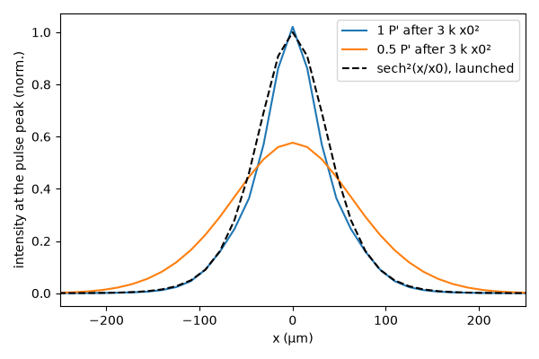
From the line tutorial: at the soliton power the beam keeps its \(\operatorname{sech}^2\) profile over three diffraction lengths; at half of it, the beam diffracts.#
Reading the output#
A free-space run writes the same output as any other, with the spatial axes, weights and
units in its metadata. The processing and plotting functions take it directly; the
fluence at a plane is spatial_fluence(), which takes the field
and the measure of its plane, a SpatialFlux resolved in the
medium at that position:
from solprop.spatial import SpatialFlux, spatial_fluence

exit_plane = run.planes()[-1]
flux = SpatialFlux.resolve(grid, space, argon, z=exit_plane.z)
fluence = spatial_fluence(exit_plane.field, flux)  # J/m², at space.r
print(f"peak fluence at the exit: {float(fluence.max()):.3g} J/m²")
The default statistics of a spatial run are the energy, the on-axis and peak
intensities, the beam radius, the full width and the on-axis spectrum
(default_spec("radial"), default_spec("free")); the
statistics catalogue defines each, and the model page
says how the widths are measured.
Where it runs#
Radial, Cartesian and line runs execute on numpy_ref, numba_cpu and the native
backend’s CPU build; its CUDA build runs them too. A Cartesian run’s memory grows
as \(n_x n_y n_t\), and the backends chapter says how it is budgeted.
The thread pools a free-space run uses, including its separate transverse FFT pool, are
on the model page under
CPU execution settings.
Limits#
The radial grid represents no azimuthal structure: a beam that breaks into several filaments, or is not round, needs the Cartesian grid.
A medium that varies along z — a pressure profile — is accepted on the radial grid only, when it meets the adiabatic certificate; the Cartesian and line grids take a constant medium.
The line is uniform in y: no collapse, no critical power, and no instability in y.
The critical power is the Townes value for a monochromatic, paraxial, Kerr-only beam. It orders a run, but it does not predict where a pulse with plasma will collapse.