Choosing a propagation model

Begin with the physical question. A calculation needs a propagation equation, a temporal description, and a way to represent the transverse field. These are related choices: the GNLSE uses an envelope and one effective area, while the UPPE can retain an optical field and a resolved transverse description.

The capabilities overview describes what solprop can calculate. The spatial introduction is a visual starting point; spatial decompositions gives the assumptions, boundaries and normalisation of each choice. After choosing a model, continue to grids, pulses and running a simulation.

For a first complete calculation, follow the multimode RDW lesson, N = 3 soliton, or one of the free-space lessons. Guide snippets illustrate individual choices; full propagation and interpretation belong to those lessons and the worked examples.

What there is

The main guided propagation routes are listed below. Free-space routes follow in the spatial overview. They share the grids, the pulses, the stepper, the output files and the backends; they differ in what a mode is.

route	entry point	a mode is	use it for
mode-averaged GNLSE	prop_gnlse	an effective area and a dispersion, or a declared \(\gamma\)	a single-mode fibre or a single mode of anything, fast; an envelope
mode-averaged gas-filled mode	prop_capillary(..., mode_average=True), prop_waveguide(..., mode_average=True)	one gas-filled mode’s effective area and dispersion, with the gas’s density, Kerr, Raman and plasma	a quick single-mode capillary run, or a comparison with Luna.jl’s default
capillary / supplied gas-filled modes	prop_capillary, prop_waveguide(modes, ..., gas=...)	a transverse scalar profile of a gas-filled hollow guide on a shared quadrature	gas-filled capillaries, antiresonant fibres, rectangular guides, hollow planar (slab) guides per unit width, tabulated modes
planar guide resolved in y	prop_planar(grid, PlanarGrid(modes, radius_y, n_y), ...)	a slab mode in x on every sample of a periodic y axis	planar compressors with a beam of finite height: self-focusing and modulational instability in y; energies in J
coherent wall	prop_capillary(..., wall=CoherentWall(...))	the capillary’s HE_1m channels (or one azimuthal order’s two families) coupled through the glass	multimode capillaries whose higher modes carry energy, straight, tapered or in a pressure gradient
general modal	prop_waveguide((), ..., provider=guide)	a provider’s own three-component E and H at every frequency, on its own nodes	solid-core fibres: step-index with vector modes, graded-index multimode, declared polarisation bases

Spatial decompositions sets these routes beside the free-space grids, one cross-section figure each, with the boundary condition, the symmetry each assumes and when it stops being valid.

Which one? A hollow guide filled with gas is the capillary route; add the coherent wall when linear coupling through the boundary matters to the retained modes, even if only the fundamental mode is populated initially. A multimode capillary taper converts between its modes whether or not the wall is declared (the taper coupling, on by default); the wall adds the coherent loss of the modes the taper fills. A solid-core fibre whose modes you want as they are — vector, frequency-dependent, with the longitudinal field — is the general modal route; a single-mode solid fibre whose only property that matters is \(\gamma\) and \(\beta(\omega)\) is still prop_gnlse, and much faster.

What each route models, pictured

Each figure is a cross-section, drawn to scale from the package’s own modes and node rules: the guide, the nodes the run evaluates its nonlinear response at, and the fields it propagates. The solid-core fibres and the capillary’s coherent wall have their own figures in their chapters (solid-core fibres, multimode capillaries); all of them, with each decomposition’s expansion, boundary and limits, are on spatial decompositions.

Mode-averaged (prop_gnlse, or prop_capillary(..., mode_average=True) for a gas-filled mode): the mode is replaced by a uniform disc of the same effective area.

The effective area preserves the single-mode cubic overlap. A mode-averaged plasma response samples an effective field; a resolved calculation samples the local field across the core, including its larger on-axis value.

A multimode gas-filled capillary (prop_capillary(modes=N)): the HE_1m modes on a radial rule, each node standing for a ring.

HE_1m modes have an azimuthally symmetric magnitude, so one azimuthal node carries the whole \(2\pi\). A set with azimuthal structure (TE_01, HE_21, …) takes a full polar rule instead.

An antiresonant hollow-core fibre (prop_capillary(..., lattice=TubeLattice(...))): the tubes set the index and the loss through Vincetti’s model; the propagated field is the core’s.

A single-ring fibre with six tubes around a 15 µm core. The field the run propagates is Marcatili’s, truncated at the core radius.

A rectangular hollow guide (prop_waveguide(modes, ..., gas=...) with RectMode): two wall pairs, on a Cartesian rule.

The polarisation decides which wall pair sees the TE-like and which the TM-like reflection.

A hollow planar guide, uniform in y (SlabMode, ModeCollection.slab): one wall pair and a free direction, so every energy is per metre of y.

The gap of a planar compressor, 127 µm between silica plates.

A planar guide resolved in y (prop_planar with a PlanarGrid): the slab modes in x on every sample of a periodic y axis, so a beam of finite height can self-focus and break up across the guide.

Slab modes in x on every y sample; y is periodic, with an absorbing collar.

What that buys is the physics that limits a real planar compressor. In the planar compressor worked example, an 8.7 mJ beam seeded with noise breaks up across y by modulational instability as it propagates:

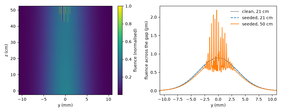
The fluence across y along the guide (left) and at two distances (right). A clean beam stays smooth; a seeded one breaks up once the B integral is large enough.

What each model gets exactly, and what it approximates

The table distinguishes the equations retained by each model from their approximations. Numerical accuracy still depends on resolution and tolerance. Quoted departures are results of particular comparisons, not general error bars.

model	exact	approximate, and how well
general modal route (chapter, model)	the vector field and the full three-component Kerr contraction at every node, per region; the real-field cubic including the third harmonic; the true-power normalisation (no \(\sqrt{\operatorname{Re}n_{\rm eff}}\) anywhere); the silica tensor Raman response	the provider’s own discretisation (a graded-index core is P1 finite elements, second order in the element count); the frequency interpolation between the guide’s knots, gated at gram_atol (1e-4) where the pulse is and warned about elsewhere; no transverse-resolution alarm during a run
step-index provider	the exact vector HE/EH/TE/TM modes of a circular step-index fibre at every frequency	a constant-index or Sellmeier material, no material loss (a complex permittivity is refused)
graded-index provider	the TE₀/TM₀ vector sectors, and an LP sector	family="LP" is weak guidance (permittivity contrast ≤ 0.02, no \(E_z\)); hybrid HE/EH graded-index sectors are refused
declared basis (chapter)	a unitary change of an exactly degenerate block (e.g. circular polarisation); a split block propagated as a coupled flow	a rotated channel of a split block reports the block’s mean \(n_{\rm eff}\), which is not a propagation constant (the block beats); zdw is withheld there
coherent wall (chapter, model)	the condensed Robin boundary of the retained HE_1m set; each channel’s loss rate departs from Marcatili’s by the relative amount \(-(4N^2t^2 + u_m^2/2(ka)^2)\), with \(N\) retained channels and \(t = v_n/k_0a\) as on the model page — e.g. \(1.2\times10^{-5}\) for one channel of a 125 µm bore at 800 nm	quasi-static and paraxial: the three validity ratios are recorded and the run warns within a factor ten of the limit and refuses above it
vector (TE/TM) wall	each family’s own impedance, the \(\mathrm{HE}\leftrightarrow\mathrm{EH}\) coupling by the wall’s anisotropy	grazing-impedance boundary; checked against the exact vector Maxwell roots family by family (to between \(5\times10^{-6}\) and \(5\times10^{-5}\) at 800 nm), but not against a resolved-cladding solve of a mixed state, which is a known limitation
taper and gradient (chapter)	the frozen-section split is a rearrangement, not an approximation (the residual is evaluated exactly); the taper connection of the capillary’s \(J_0\) basis; each channel’s own normalisation	the step error, controlled by the stepper; CF4’s flow error is invisible to the controller
moving solid guide (chapter, model)	the mode fields re-solved along z at the degree a held-out check demands, the moving synthesis and projection maps, the solid-mode connection in the frozen-residual flow	the frozen-section step error, controlled by the stepper; a strong taper needs short steps or sections= (the advisory step warns)
planar guide resolved in y (model)	slab modes in x times an FFT in y, exact (non-paraxial) in y, each channel’s complex wall term in its longitudinal wave number; a field uniform in y is the slab run	the slab’s first-order wall model; constant gap and fill; one polarisation family (TE or TM)
hollow planar (slab) guide (model)	Laakmann–Steier’s one wall pair with the filled-core contrast; \(N\) and \(A_{\rm eff}=4a/3\) per unit width; the Gaussian launch’s projection onto the slab modes	first order in \(p\lambda/4a\); uniform in y: powers and energies are per metre of y, and self-focusing, filamentation and modulational instability in y are absent (they set a real compressor’s energy limit); a taper follows each mode adiabatically
line free space (model)	the Cartesian exact operator and FFT on one x axis with \(k_y = 0\); energies J/m and powers W/m per metre of y; the (1+1)-D Gouy phase, amplitude law and sech soliton	constant media only; uniform in y: no collapse and no critical power, and a sheet beam’s instability in y is absent

Which backend runs what

Every backend refuses, by name and before allocating anything, a problem it does not run; nothing falls back. “Qualified” in the GPU column means the parity and repeatability tests pass on a data-centre NVIDIA GPU (CUDA) and an AMD Instinct GPU (HIP).

	numpy_ref	numba_cpu	native CPU	native GPU (CUDA/HIP)
general modal route (all its responses, declared bases, a split block as a coupled flow)	yes	yes	yes	qualified
a moving solid guide (moving maps beside the frozen-residual flow)	yes	yes	yes	qualified
coherent wall, scalar and TE/TM, straight, tapered or in a gradient (method="frozen_residual"), and the taper coupling of a multimode capillary without a wall	yes	yes	yes	qualified
CoherentWall(method="cf4")	yes	refused by name	refused by name	refused by name
a varying guide whose linear operator or nonlinear prefactor takes the general z table rather than an expansion in the medium’s parameters (e.g. a moving dispersion, the adiabatic opt-out taper_coupling=False of a multimode taper whose expansion does not resolve, or a mixture of three or more species on independent density paths)	yes	yes	yes	refused by name
a hollow planar (slab) set, constant gap or tapered, mode-averaged or multimode	yes	yes	yes	runs as any mode set; not separately qualified
a line free space uniform in y (LineGrid, per metre of y)	yes	yes	yes	qualified (CUDA)
a planar guide resolved in y (PlanarGrid)	yes	yes	yes	not qualified
a frequency-dependent electronic response, MaterialSelection(electronic="symmetric-kerr") or "gas-polynomial" (model), on every route but the GNLSE	yes	yes	yes	qualified
a noise model beside a coupled flow; a coupled flow in a lockstep batch	refused	refused	refused	refused

backend="auto", the default, is native where it is installed and numba_cpu otherwise, and it never falls back: a problem the native backend refuses is refused, by name, and you choose numba_cpu for it explicitly. Whether the native backend runs on the CPU or on a GPU is decided by how it was built. The backends chapter compares the backends and budgets memory; the native backend says how to build it, locally or for a GPU; performance covers threads and tuning. Every compiled backend agrees with numpy_ref, the oracle, to a rounding bound derived before any measurement; the measured departures are a few units in the last place (the bounds are in the backend design notes).

What the worked examples show

example	route	what it shows
A pressure-gradient soliton compressor	coherent wall, gradient	soliton self-compression to about 2 fs in a decreasing pressure gradient, against a constant fill, and a pressure scan
A tapered capillary: compression, a dispersive wave and mode conversion	taper coupling, with and without the coherent wall	the taper’s own linear mode conversion, isolated at a nanojoule and compared with the adiabatic opt-out; then compression and a dispersive wave pushed into the ultraviolet by the taper
Radially and azimuthally polarised pulses: the vector wall over a metre	TE/TM wall	the four families’ losses across the band; radially against azimuthally polarised compression; \(\mathrm{HE}_{11}\to\mathrm{EH}_{11}\) conversion over a metre
Spatiotemporal propagation in a graded-index multimode fibre	general modal	a graded-index multimode fibre launched with a declared Gaussian beam: self-imaging, geometric parametric instability, energy exchange between the channels
A tapered graded-index fibre: adiabatic and abrupt mode conversion	general modal, moving guide	a tapered graded-index fibre: \(\mathrm{LP}_{01}\to\mathrm{LP}_{02}\) conversion from abrupt to adiabatic against Love’s criterion, the fields at entrance and waist, self-phase modulation and the Kerr lens in the waist
A planar hollow-waveguide compressor	planar guide resolved in y	Arnold’s and Akturk’s planar compressor (127 µm gap, argon, 8.7 mJ): modal shares, loss against the closed form, compression at the beam centre, the duration and fluence across y, and a noisy beam breaking up by modulational instability as the B integral grows

The worked examples run at full size. Each page reports its measured runtime and backend; the cost depends on the problem, resolution and hardware. Start with the introductory lessons, then use these comparisons when you need their additional physics or parameter scans.