Multimode capillaries: the coherent wall, tapers and gradients

This chapter is for multimode runs of a gas-filled capillary: when the higher HE_1m modes matter, how to declare the coherent wall that couples them, how tapers and pressure gradients are handled, and what each option costs. The derivation, the limits and every check are on the model page, the coherent wall; this chapter is how to use it. A single-mode run whose response is expensive – an atomic response with one atom per node – chooses its radial nodes as described in radial nodes for expensive responses.

A gas-filled capillary is propagated on its Marcatili modes. On the ordinary route each HE_1m mode loses energy through the wall on its own: the loss is incoherent, and the wall never moves energy from one mode to another. That is right when the modes that carry energy are far apart in propagation constant compared with the wall’s coupling, and wrong when they are not. Separately, a guide whose bore varies along its length changes the shape of its own modes, and that converts energy between them whatever the wall does. Two options carry these effects:

• the coherent wall, wall=CoherentWall(): the outgoing boundary condition at the glass, condensed onto the retained modes, which couples every mode to every other with a definite phase;

• the taper coupling, on by default for a multimode capillary whose radius varies: the connection \(\langle\psi_m|\partial_z\psi_n\rangle\) between the local modes, which converts energy between them as the bore changes. With a wall it is part of the wall’s flow; without one it is carried alone.

The same modes and node rule, two wall models. Left, the ordinary Marcatili wall: each mode has its own loss and nothing moves between them. Right, the coherent wall: the outgoing boundary condition, condensed onto the modes through each mode’s slope at the wall, couples every pair.

When to use it

• More than one mode carries energy that matters. A launch that is not a perfect HE_11, strong self-focusing or ionisation that fills the higher modes, a mode converter: the wall’s exchange between modes is then part of the physics. How a beam focused through gas is coupled into the modes is in coupling simulations and the capillary coupling tutorial.

• The bore tapers and the wall’s loss matters: a multimode taper converts between its modes whether or not a wall is declared — the taper coupling is on by default (below) — and the wall adds the coherent loss of the modes it fills.

• Radial and azimuthal polarisation, or a hybrid mode’s partner family: the vector wall, impedance="te_tm", gives the glass its two impedances, so TE_0m and TM_0m keep their own losses and HE_1m couples to EH_1m.

A single-mode run, or a multimode run in which only HE_11 matters, gains nothing from the wall: leave wall=None, the default.

A straight bore

Pass wall=CoherentWall() to prop_capillary, with modes=N: the wall needs the contiguous set HE_11 to HE_1N, which is what an integer builds. The snippets on this page run ten fixed steps over a fifth of a millimetre, which is what makes them finish in seconds; the worked examples run the same calls over metres. The keywords they share are gathered in common: a fixed schedule of ten steps, a three-mode set launched in HE_11, and no plasma or Raman response.

import warnings

import numpy as np

from solprop.boundaries import absorber
from solprop.driver import prop_capillary
from solprop.grid import FieldGrid
from solprop.modes import CoherentWall
from solprop.processing import energy
from solprop.stepper import FixedSchedule, RungeKutta

length, steps = 2e-4, 10
grid = FieldGrid.from_limits(length, 800e-9, (400e-9, 1.6e-6), 300e-15)
common = dict(
    lambda0=800e-9,
    grid=grid,
    fwhm=30e-15,
    energy=1e-9,
    modes=3,
    n_save=6,
    # The absorber acts inside every stage, so a strong collar limits the step: this
    # one is weak enough for twenty-micrometre steps.
    absorber=absorber(grid, boundary_length=1e3),
    schedule=FixedSchedule(np.full(steps, length / steps)),
    dz_max=length / steps,
    dz_init=length / steps,
    plasma=False,
    raman=False,
    progress="none",
)
walled = prop_capillary(50e-6, length, "He", 1.0, wall=CoherentWall(), **common)
plain = prop_capillary(50e-6, length, "He", 1.0, **common)

for name, run in (("coherent wall", walled), ("incoherent", plain)):
    shares = np.asarray(energy(run, plane=-1)) / float(np.sum(energy(run, plane=0)))
    print(f"{name:14s}", ", ".join(f"{share:.2e}" for share in shares))

Launched into HE_11 alone, the walled run puts energy into HE_12 and HE_13; the incoherent one cannot, and what it leaves there is the Kerr overlap between the modes alone, many orders of magnitude smaller.

What the wall replaces. It is the loss model: loss= must stay True (a scale, a curve or False beside a wall is refused rather than silently dropped), and model="reduced" is refused because the condensation inverts the full model’s eigenvalue. A tube lattice (lattice=) is refused beside it: an antiresonant fibre’s loss is its tubes’ resonances, not a boundary condition at one radius. Two polarisations, a noise model and a fused batch are refused too, each by name.

Validity. The condensation is quasi-static and paraxial. Three dimensionless ratios are computed for the highest retained mode over the band the run scores — the requested wavelength limits (grid.inband_mask), where the step’s error is measured — and recorded; the run warns when one comes within a factor ten of CoherentWall.validity_limit (0.25), naming it, and refuses above it. The spectral collar a field grid adds below that band, down to half its lowest frequency, still carries the block but is absorbed rather than scored, so it does not count: every ratio grows with the wavelength, and over the collar each would be about twice its in-band value. Which ratio is met first depends on the case. For small bores it is often the quasi-static ratio \(2N/|ak_{\rm eff}|\), largest at the band’s longest wavelengths and for many modes. On a broad band it can be the vacuum or transverse ratio: a 125 µm helium bore at 1 bar over a 200 nm to 2 µm band admits N = 31 and refuses N = 32 on the vacuum ratio (0.2531). Fewer modes, a larger bore or a narrower band move all three; the warning and the refusal name the ratio that set them.

The step. A run with a wall needs dz_max: the interaction picture inverts the coupled flow over each step, and over the default cap of half the fibre a lossy multimode block amplifies the source by more than the flow admits (CoherentWall.condition_limit, 1e4). The refusal names the step and the frequency; a few millimetres is typical for a metre of fibre.

Reading what the wall was

The run’s record carries the block as a flow entry, so a file says what it propagated:

flow = walled.metadata.modal["flow"]
print(flow["model"], "|", flow["n_sections"], "section(s),", "n_deg", flow["n_deg"])
print(
    "validity ratios:",
    flow["transverse_ratio"],
    flow["vacuum_ratio"],
    flow["quasi_static"],
)

n_sections and n_deg describe the sectioning along z (one section and one coefficient for a straight bore); connection says whether the taper’s connection was carried; advisory_step is the step a declared dz_max or schedule is warned against. The whole table is on the model page.

Tapers and pressure gradients

A taper is a radius profile, a gradient a pressure pair or profile; both are declared as they always are (Profiles along the fibre). A pressure pair or (z, p) table is built into a steady flow that follows the bore: along a taper \(p^2\) is linear in \(\int a^{-4}\,dz\), so a narrow waist carries most of the pressure drop, and an end pumped to vacuum is choked — it takes the pressure at which the laminar throughput equals the sonic one, not zero (solprop.gasflow.steady_fill()). A declared end below that value is raised to it, with a log saying so; vacuum_end="floor" keeps the declared ends instead — it concerns the ends only, and a taper’s fill still follows the bore. Every mode that declares a core_radius (every MarcatiliMode subclass, a TabulatedMode built from arrays included) is taken as a circular bore of that radius. The fill warns (GasFlowWarning) when the flow is not laminar (a peak Reynolds number above 2000, at a taper’s waist) or not a continuum (a Knudsen number above 0.01 at a stage’s mean pressure and narrowest bore, or more than 1 % of its gas above 0.1); a choked helium exit, transitional over micrometres, is only logged. A PressureGradient supplied directly is used as given, and warns if it was built without the bore of a guide that varies.

A gas temperature that varies along the fibre is a profile too, temperature= in K: the density follows \(\rho(p(z), T(z))\), the steady flow is weighted by the viscosity times the temperature (a warm stretch carries more of the drop), a choked end takes its own temperature’s viscosity and sound speed, and the rotational Raman populations of a molecular fill take one reference temperature, with a warning (Profiles along the fibre, The Raman response). A constant profile is the number.

The steady flow of any fill is reported by solprop.gasflow.flow_report(): per stage the PV throughput (in Pa m³/s, with throughput_mbar_litres_per_second and throughput_slpm for the vacuum units), the mass flow, the peak Reynolds number and where it is, the Knudsen numbers at both ends, and whether each outer end is choked:

from solprop.gasflow import flow_report, steady_fill

fill = steady_fill("He", [0.0, 3.0], [5.0, 0.0], radius=125e-6)
print(flow_report(fill, "He", radius=125e-6))

A taper from 50 to 40 µm, drawn along z. The nodes ride the bore and the modes change shape with it; what moves energy between them is the connection.

How a varying guide is propagated. With a wall, the run is cut into sections at the profile’s corners, the complete generator of the coupled modes (their propagation constants and the wall’s coupling) is frozen at each section’s midpoint and integrated exactly, and everything the freezing leaves out — the generator’s variation along the section and, on a taper, the connection \(C_{mn} = (a'/a)\,2s_ms_nu_mu_n/(u_m^2 - u_n^2)\) for \(m \ne n\), with \(a\) the core radius, \(u_m\) the \(m\)-th zero of \(J_0\) and \(s_m = \operatorname{sgn}J_1(u_m)\) — is put back exactly as an explicit term in the Runge–Kutta source. Freezing is therefore a rearrangement, not an approximation: one section per interval and four agree to \(2\times10^{-10}\).

The two runs below, a taper from 50 to 40 µm and a pressure gradient, are a fifth of a millimetre long, far too short to hold a pressure difference as a laminar flow (the gradient’s end would choke at about 0.88 bar, and the fill warns): vacuum_end="floor" imposes the declared ends, which is what this numerical demonstration wants.

At full size, a pressure gradient is how a capillary compresses a pulse to a few femtoseconds. The gradient compressor worked example runs two metres of a 125 µm helium-filled bore from 0.8 bar to vacuum, four modes with the coherent wall:

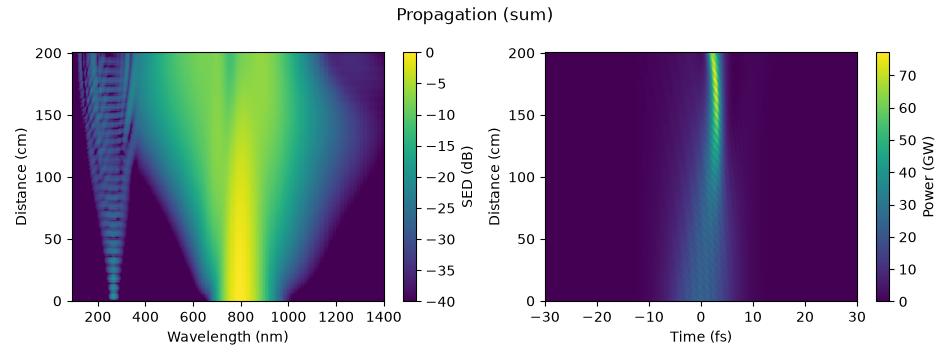
The spectrum (left) and the power (right) along the gradient, summed over the modes: a 10 fs, 250 µJ pulse compresses to its highest peak power near the exit.

from solprop.profiles import PiecewiseLinear

taper = PiecewiseLinear.from_stages(
    (0.0, 6e-5, 1.4e-4, 2e-4), [50e-6, 50e-6, 40e-6, 40e-6]
)
tapered = prop_capillary(taper, length, "He", 1.0, wall=CoherentWall(), **common)
gradient = prop_capillary(
    50e-6, length, "He", (1.0, 0.2), vacuum_end="floor", wall=CoherentWall(), **common
)

for name, run in (("taper", tapered), ("gradient", gradient)):
    flow = run.metadata.modal["flow"]
    shares = np.asarray(energy(run, plane=-1)) / float(np.sum(energy(run, plane=0)))
    print(
        f"{name:9s} connection={flow['connection']}, sections={flow['n_sections']};",
        ", ".join(f"{share:.2e}" for share in shares),
    )

The taper converts several per cent of the launch into HE_12 and HE_13 over its 80 µm transition, and that — not a larger attenuation at the smaller radius — is what a non-adiabatic taper costs, because the modes it fills are the lossier ones. A gradient in a fixed bore moves no mode shape, so it carries no connection.

The taper coupling without a wall

A multimode capillary whose radius varies carries the connection by default, with or without a wall and lossless or not: the same frozen-residual flow as the walled taper, with the wall term zero and each mode’s own propagation constant — its Marcatili index, with whatever model= and loss= it declares — on the diagonal. A lossless capillary (loss=False) is then a crude model of a low-loss anti-resonant fibre whose small-core tapers convert as they should. taper_coupling=False is the explicit opt-out to the adiabatic route, on which each mode follows its local shape and no power moves between them:

lossless = dict(common, loss=False, cladding=1.45)
coupled = prop_capillary(taper, length, "He", 1.0, **lossless)
adiabatic = prop_capillary(taper, length, "He", 1.0, taper_coupling=False, **lossless)

for name, run in (("taper coupling", coupled), ("adiabatic", adiabatic)):
    shares = np.asarray(energy(run, plane=-1)) / float(np.sum(energy(run, plane=0)))
    print(f"{name:15s}", ", ".join(f"{share:.2e}" for share in shares))
print(coupled.metadata.modal["flow"]["model"], adiabatic.metadata.modal)

The coupled lossless run keeps the launched power (the connection is antisymmetric in the true-power amplitude) and moves several per cent of it out of HE_11; the adiabatic one leaves the higher modes empty. The record says which ran: modal.flow.model is "taper coupling", and a file written with it is not resumed by the opt-out.

The tapered capillary worked example isolates the conversion over a metre of fibre — 50 cm at 100 µm, a 20 cm taper to 60 µm, 30 cm at 60 µm — at a nanojoule, where nothing is nonlinear:

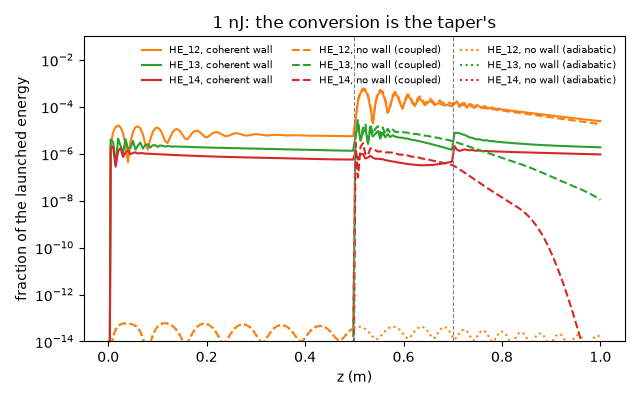
The energy in the higher modes along the fibre, launched in HE_11. With the wall (solid) or with the connection alone (dashed) the taper converts at its corners; the adiabatic opt-out (dotted) converts nothing.

What applies it, and what does not:

• Which sets. The contiguous HE_11 to HE_1N block of plain capillary modes, N >= 2, on a varying radius (taper_coupling_block()). One mode needs no connection, and a constant bore has none — a pressure gradient included, which changes each mode’s index, carried on its own diagonal, but not its \(J_0(u_m r/a)\) shape. A set the connection is not derived for (a tube lattice, a sparse or mixed set, tabulated modes) stays adiabatic and warns (AdiabaticTaperWarning).

• What it refuses, by name and naming the opt-out: an envelope grid (no coupled flow is built on its frequency axis), a noise model, a second field component, and a radius profile without an analytic slope (the connection is \(a'/a\)). Beside a wall, taper_coupling=False is refused: the wall carries the connection.

• The step. As with a wall, the interaction picture inverts the flow over each step, and a lossy block amplifies the source by the spread of the modes’ attenuation over it: over the default cap of half the fibre, with a band reaching the infrared, that exceeds what the flow admits, and the run is refused naming the step. Declare dz_max (a few millimetres for a metre of fibre). A lossless block has no such spread. A declared step above the flow’s advisory step warns, advisory only.

• The cost. A step costs about 1.4 to 1.6 times the adiabatic one at three modes and about twice at eight on the CPU backends, more at many modes; translation is dearer too, once per run.

Every mode keeps its own normalisation. On a varying guide a mode’s amplitude is renormalised as its effective index changes along z. The part every mode shares is the lowest mode’s, carried in the diagonal propagator; the rest of each mode’s own, \(-\tfrac12\,d\ln(w_n/w_1)/dz\) with \(w = \operatorname{Re}n_{\rm eff}\), is carried in the flow’s diagonal, from the closed-form slope (dneff_dz()), never a difference. Nothing is declared for it; it is why the upper modes’ amplitudes are good to the step error on a taper: giving every mode the lowest mode’s normalisation instead would move the upper modes of the 50 to 40 µm taper above by up to \(5\times10^{-4}\) at the edge of the band. What the record holds is the true-power amplitude of every mode: energy of a mode is that mode’s energy.

The band you ask for is the band that is coupled. The varying part of the wall and the taper’s conversion are integrated on the requested wavelength band, the bins the step controller checks; in the spectral collar just outside it (to twice the longest wavelength and a tenth beyond the shortest) each section’s midpoint wall alone carries the field. Content there is not a result either way – the collar absorbs it – and it reaches the band only through the nonlinear response; widen wavelength_limits if the conversion at those wavelengths matters to you. (Applying the explicit residual in the collar too would be unstable there: the step controller does not score those bins, so it would not shorten the step to hold it.)

Two rules the profile must follow. A radius or density profile must have an analytic slope (a FromCallable without one is refused: a difference of samples is noise), and every mode must declare the same profiles. A fixed schedule must land on every corner of the profile — the ten equal steps above do, because the corners are multiples of the step, and FixedSchedule.uniform(z_start, z_end, dz, hard_kinks=corners) builds one that does for any corners; adaptive stepping lands on corners by itself; a schedule that comes near a corner without landing on it is refused.

The frozen split or CF4. CoherentWall(method="cf4") integrates each section’s whole generator by the fourth-order commutator-free exponential instead of freezing it: no explicit residual and no advisory step, but a flow error the step controller cannot see, a run at most fourth order, and a step 3.3 times dearer. It is the more accurate only for steps beyond the frozen split’s advisory limit, so prefer the default; use CF4 when you must take steps longer than advisory_step and have checked the answer by halving them. It runs on numpy_ref only and with the Runge–Kutta march only (integrator=RungeKutta(); the default Adams method refuses it), is refused on a guide that does not vary, and is admitted only where its growth guard (growth_limit, default 2) holds — with fallback="frozen_residual" a section the guard rejects is integrated by the frozen split instead of refused:

cf4 = prop_capillary(
    taper,
    length,
    "He",
    1.0,
    backend="numpy_ref",
    integrator=RungeKutta(),
    wall=CoherentWall(method="cf4", fallback="frozen_residual"),
    **common,
)
difference = np.max(np.abs(cf4.planes()[-1].field - tapered.planes()[-1].field))
print(
    f"CF4 against the frozen split: {difference / np.max(np.abs(tapered.planes()[-1].field)):.1e}"
)

The vector wall: radial and azimuthal polarisation

CoherentWall(impedance="te_tm") gives the wall’s tangential and normal fields their own impedances. The block is one azimuthal order \(\nu\) — its two radial families, each contiguous from \(m = 1\) — declared as a supplied mode set: TE_0m and TM_0m for \(\nu = 0\) (which the wall does not couple, and either may be retained alone), HE_νm and EH_νm for \(\nu \ge 1\) (which it does, through the impedances’ difference). A negative azimuthal index is this package’s spelling of the EH family.

from solprop.modes import MarcatiliMode

order_one = [
    MarcatiliMode(50e-6, "He", 1.0, n=order, m=radial)
    for order in (1, -1)
    for radial in (1, 2)
]  # HE_11, HE_12, EH_11, EH_12
vector = prop_capillary(
    50e-6,
    length,
    "He",
    1.0,
    wall=CoherentWall(impedance="te_tm"),
    **{**common, "modes": order_one},
)
shares = np.asarray(energy(vector, plane=-1)) / float(np.sum(energy(vector, plane=0)))
print("HE_11, HE_12, EH_11, EH_12:", ", ".join(f"{share:.2e}" for share in shares))

A supplied set carries its own geometry: the positional radius must agree with every mode’s, and model, loss or cladding away from their defaults must be the modes’ own; a disagreement is refused by name rather than silently ignored. A TE_0m or TM_0m launch has no field on the axis, so the ionisation table’s default range is read from the peak over the axis and the run’s own transverse nodes, where the plasma is evaluated; ionisation_field_range= still overrides it (worked example 03 declares one). The vector wall carries a taper and a gradient exactly as the scalar one does, with each family’s own connection; CF4 is admitted beside it.

A set with azimuthal structure is evaluated on a full polar rule rather than the radial one, with both transverse components at every node:

The azimuthally polarised \(\mathrm{TE}_{01}\) mode on the polar product rule.

In the vector wall worked example the two families compress differently, because the glass treats them differently:

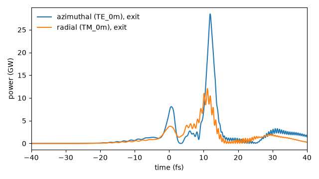
The exit pulses of an azimuthally (TE_0m) and a radially (TM_0m) polarised launch, each with three radial orders and the vector wall.

Backends

All three backends run the wall — scalar and TE/TM, straight, tapered or in a gradient — and the taper coupling without one, with the frozen split; CF4 is numpy_ref’s alone. The adiabatic opt-out of a multimode taper (taper_coupling=False) puts every mode on its own row of the linear operator, and where that expansion does not resolve (a metre of kinked taper, for instance) it takes the general z table, which every CPU backend runs, the native CPU build included, so backend="auto" runs such a comparison; the native backend’s GPU builds refuse it by name, naming the CPU backends. On the capillary’s small grids a locally built native backend is the fastest backend at one to four threads; see backends, the native backend and performance.