4. Waveguide modes

Chapters 2 and 3 used the word mode as if its meaning were obvious. For a propagation code it is a precise contract: a transverse field, a complex propagation constant at every frequency of the grid, its frequency derivative, and a normalisation that makes the amplitude mean something. This chapter states that contract and then works through the guides solprop provides.

Most of the guides solprop is used for are hollow and filled with gas. They do not strictly guide light at all. Their modes leak through the wall, which is why their loss and dispersion come from asymptotic, grazing-incidence models rather than from an exact eigenvalue problem. The solid-core fibres are the opposite case: their modes are exact solutions of a vector eigenproblem, and the difficulty lies elsewhere. By the end of the chapter you should know where each model’s numbers come from, what each one assumes, how far each has been checked, and why the radius of a capillary is the number to watch.

4.1 What a propagation code needs from a mode

In the modal UPPE of §2.5 and §2.9, a mode enters in two places. The linear operator needs its complex effective index \(n_{\rm eff}(\omega)\), through

\[ \beta(\omega)=\frac\omega c\operatorname{Re}n_{\rm eff},\qquad \alpha(\omega)=\frac{2\omega}c\operatorname{Im}n_{\rm eff}, \]

and the frame needs the analytic derivative \(\mathrm dn_{\rm eff}/\mathrm d\omega\). The nonlinear term needs the transverse field, to synthesise the field at the points where the response is evaluated and to project the response back. solprop’s mode classes supply exactly these: an index, its derivative with respect to frequency (and, for a guide that changes along \(z\), with respect to its parameters), a transverse profile and an effective area (waveguide modes).

Remember the convention of Chapter 1: \(\operatorname{Im}n_{\rm eff}>0\) is loss, and \(\alpha\) is a power attenuation coefficient, so the field decays as \(e^{-\alpha z/2}\). The classic waveguide papers often quote the field coefficient instead. Marcatili and Schmeltzer (1964, Eq. 37) define \(\alpha=\operatorname{Im}\gamma\) through \(\mathrm dP/\mathrm dz=-2\alpha P\), and the antiresonant-fibre papers write \(8.686\operatorname{Im}\gamma\) in dB/m. Losses in dB/m agree once that factor of 2 is accounted for, but coefficients in m⁻¹ do not.

4.2 Normalisation, and what the amplitude means

A modal amplitude is only meaningful once the mode’s field is normalised. Kolesik and Moloney (2004, Eq. 12) normalise by the Poynting flux. solprop’s scalar routes (the capillary, the antiresonant, rectangular and planar guides, and tabulated hollow modes) use a vacuum normalisation instead,

\[ \frac{\varepsilon_0c}{2}\int|e|^2\,\mathrm dA=1, \]

so that an internal amplitude \(a\) in \(\sqrt{\rm W}\) multiplies a profile in V/m per \(\sqrt{\rm W}\) (polarisation). For the capillary this is exactly the power that Marcatili and Schmeltzer (1964, Eq. 42) give for a unit-amplitude mode in the core. The true power carried by the mode is not \(|a|^2\), though. A mode with effective index \(n_{\rm eff}\) carries a power \(\operatorname{Re}n_{\rm eff}\,|a|^2\) for the same field, because its magnetic field is larger by that factor. solprop therefore saves the true-power amplitude

\[ b=\sqrt{w}\,a,\qquad w=\operatorname{Re}n_{\rm eff}, \]

whose spectral energy and total energy are the mode’s (power, energy and intensity). For a narrow band or a constant index, \(|b(t)|^2\) is the power. For a broadband pulse whose \(w\) varies with frequency it is not quite: the temporal Poynting trace that solprop’s statistics report is \(\operatorname{Re}[a(t)a_w^*(t)]\), with \(a_w\) the inverse transform of \(w(\omega)a(\omega)\), and the two share their time integral but not necessarily their peak or duration. Inputs are given in these units and outputs are reported in them. The internal \(a\) is used only inside the propagation. The \(-\tfrac12\partial_z\ln w\) term of §2.9 is what keeps \(|b|^2\) correct where \(w\) changes along the guide. For a gas at 20 bar the difference between \(|a|^2\) and \(|b|^2\) is about half a per cent, small but not negligible (watts and volts per metre).

Solid-core fibres with their vector modes use a different and more general normalisation: unit Poynting flux, through a Hermitian flux metric \(W\) computed from the electric and magnetic fields of each mode (Chapter 5). For these the power weight is one by construction.

4.3 The hollow capillary

A glass capillary filled with gas is the simplest hollow waveguide, and the one solprop’s main route is built around. The core has a lower index than the wall, so total internal reflection is impossible. The light is confined only because reflection from the wall at grazing incidence is very nearly total. Every mode leaks. What is computed is a leaky mode: a solution with a complex propagation constant that slowly loses power through the wall.

Marcatili and Schmeltzer (1964) gave the asymptotic theory for a circular guide of radius \(a\) in a wall of complex index \(\nu\), assumed infinitely thick. For \(ka\gg|\nu_n|u_{nm}\), so that the core is many wavelengths across, the transverse wavenumber in the core is \(k_ia\approx u_{nm}(1-i\nu_n/ka)\) (their Eq. 18). From it follow the propagation constant and attenuation (their Eqs. 20–21):

\[ \gamma\approx k\Big[1-\frac12\Big(\frac{u_{nm}\lambda}{2\pi a}\Big)^2\Big(1-\frac{i\nu_n\lambda}{\pi a}\Big)\Big], \qquad \operatorname{Im}\gamma=\Big(\frac{u_{nm}}{2\pi}\Big)^2\frac{\lambda^2}{a^3}\operatorname{Re}\nu_n . \]

Here \(u_{nm}\) is the \(m\)-th zero of \(J_{n-1}\), and \(\nu_n\) depends on the family of the mode: \(1/\sqrt{\nu^2-1}\) for \(\mathrm{TE}_{0m}\), \(\nu^2/\sqrt{\nu^2-1}\) for \(\mathrm{TM}_{0m}\) and \(\tfrac12(\nu^2+1)/\sqrt{\nu^2-1}\) for the hybrid modes (their Eq. 17). The hybrid factor is the mean of the TE and TM ones. Two features dominate everything that follows. The waveguide contribution to the index, \(-\tfrac12(u_{nm}\lambda/2\pi a)^2\), is negative and grows as \(\lambda^2\), so it is anomalously dispersive. And the loss scales as \(\lambda^2/a^3\): halving the radius multiplies the loss by eight.

solprop writes the model in a form that keeps a gas-filled core and does not expand the square root (the Marcatili model):

\[ n_{\rm eff}=\sqrt{\varepsilon_{\rm co}-\Big(\frac{u_{nm}}{ka}\Big)^2\Big(1-\frac{iv_n}{ka}\Big)^2}, \]

with \(\varepsilon_{\rm co}=1+\chi_{\rm gas}(\omega)\) the permittivity of the gas and \(v_n\) Marcatili’s \(\nu_n\) written with the cladding permittivity \(\varepsilon_{\rm cl}=\nu^2\). The gas-filled core is an extension: Marcatili’s core is vacuum. Its real part is the form Travers et al. (2011, Eq. 1) use for gas-filled hollow fibres. A reduced form, linear in the small quantities, is also available. It is exactly Marcatili’s Eq. 20 with the gas added. Both are asymptotic in \(1/ka\).

Some numbers fix the scales. At 800 nm in a silica capillary, the \(\mathrm{HE}_{11}\) loss is 4.9 dB/m for a radius of 62.5 µm and 0.62 dB/m for a radius of 125 µm, and the waveguide index deficit is \(-1.2\times10^{-5}\) and \(-3.0\times10^{-6}\). One bar of argon at room temperature adds about \(+2.6\times10^{-4}\) to the index, and its dispersion is normal. The balance between the anomalous waveguide term and the normal gas term sets the zero-dispersion wavelength, and the gas pressure tunes it. This is the property that makes gas-filled fibres so useful for soliton dynamics (Travers et al. 2011).

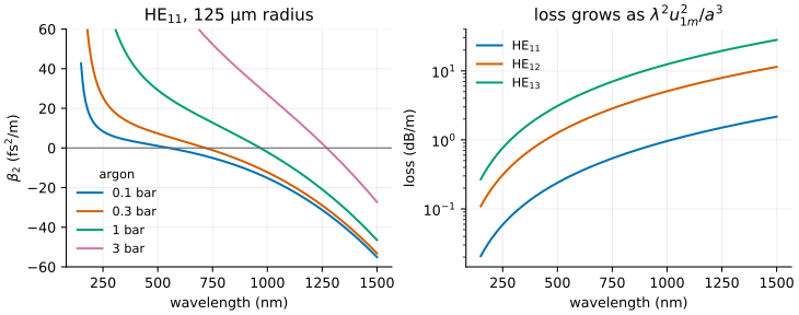
Left: the anomalous waveguide dispersion and the normal dispersion of the gas balance at a zero-dispersion wavelength that the pressure tunes, here from about 550 nm at 0.1 bar to about 1270 nm at 3 bar. Right: the Marcatili loss, rising as \(\lambda^2u_{1m}^2/a^3\). Computed with solprop’s MarcatiliMode and its default fused-silica wall by docs/primer/figures/primer_figures.py.

Radius or diameter? Marcatili and Schmeltzer, Andreasen and Kolesik, and every solprop constructor use the radius. Travers et al. (2011) and most experimental papers quote the core diameter. “A 125 µm capillary” in solprop’s documentation means a radius of 125 µm. Get this wrong and the loss is wrong by a factor of 8.

Three further details are part of the model as solprop implements it.

• Mode names. Marcatili’s \(\mathrm{EH}_{11}\) is the \(\mathrm{HE}_{11}\) of the fibre literature and of solprop. solprop spells the other hybrid family \(\mathrm{HE}_{-1,m}\), which is Marcatili’s \(\mathrm{EH}_{-1,m}\), and labels it \(\mathrm{EH}_{1m}\).

• Numerics. The quantity \(n_{\rm eff}-1\) is of order \(10^{-4}\), so it is formed directly as \(z/(\sqrt{1+z}+1)\), without subtracting 1 from a number close to 1. The frequency derivative is analytic (capillary modes and dispersion). The cladding is optmat’s causal fused-silica model by default.

• The field. The \(\mathrm{HE}_{11}\) profile is \(J_0(u_{11}r/a)\), with \(u_{11}=2.405\). Its effective area is \(1.497\,a^2\), and its on-axis intensity is 1.768 times \(P/A_{\rm eff}\) (§3.1). The profile is truncated at the wall, which is part of the large-core approximation.

Andreasen and Kolesik (2013, PRE) compared this standard “approximate leaky-mode expansion” with simulations that resolve the wall. They found that it overestimates the losses of nonlinearly reshaped pulses, so that its peak intensities come out up to 25% lower, because the instantaneous loss depends on whether the beam actually touches the wall. Chapter 5 explains how solprop’s coherent wall addresses this.

4.4 Antiresonant fibres

An antiresonant hollow-core fibre surrounds the core with a ring of thin-walled glass tubes. Each tube wall acts like a Fabry–Pérot etalon. When the wall is antiresonant for the core light, the light is reflected back into the core with very low loss. When it is resonant, the light couples out through the wall. The resonances occur near

\[ \lambda_m\approx\frac{2t}{m}\sqrt{n^2-1}, \]

for wall thickness \(t\) and glass index \(n\), an asymptotic condition that Vincetti (2016) states in terms of the normalised frequency \(F=(2t/\lambda)\sqrt{n^2-1}\). A wall of 0.5 µm has its first resonance near 1.05 µm and its second near 525 nm.

solprop’s VincettiMode is built from three papers by Vincetti and colleagues, each an empirical fit to finite-element simulations (the Vincetti model):

1. Vincetti (2016, Eq. 3) gives the minimum confinement loss of a transmission band, as a scaling law in \(\lambda^{4.5}/a^4\), the tube-wall aspect ratio \((1-t/r)^{-12}\) and the wall index.

2. Vincetti and Rosa (2019, Eqs. 2–7) multiply that floor by a sum of Lorentzians, with width 0.003 in \(F\), centred on fitted cut-offs of the tube-wall modes. This gives the high-loss bands.

3. Rosa, Melli and Vincetti (2021) extend the model to the effective index, the group-velocity dispersion and the effective area. They use an effective core radius slightly larger than the inscribed one and a dispersive Lorentzian correction near each resonance.

The propagated field is Marcatili’s \(J_0\) profile, truncated at the core radius. The tubes set the index and the loss, but the field does not resolve them.

Because the model is a fit, its domain matters. The fits were validated for wall aspect ratios \(0.05\le t/r\le0.2\), six to ten tubes, glass indices 1.44–2.42, and the first four transmission bands (Vincetti and Rosa 2019, Table 1). solprop compares the model with converged finite-element solutions of one fibre that lies outside that range. Its index is right to \(7.5\times10^{-6}\) RMS, but its loss at the edges of the band is up to 150 times too low. Its group-velocity dispersion in the first band is 18–70% too shallow toward the long wavelength edge (accuracy against a finite-element solution). For soliton dynamics, where the dispersion is the quantity that matters most, this is a real limitation. When an accurate dispersion of a particular fibre is needed, the better route is to compute or measure it and supply it as a table (§4.7).

The physics near a resonance is richer than a Lorentzian loss peak. Melli et al. (2025) show that a core mode and a cladding mode can be weakly coupled, which gives a loss peak with a crossing of the dispersion curves, or strongly coupled, which gives an anticrossing, depending on whether \(2|\kappa|\) is smaller or larger than the difference of their losses. solprop does not model this.

4.5 Rectangular and planar hollow guides

A hollow guide of rectangular cross-section, or two flat plates with a gas-filled gap, has the same grazing-incidence physics as a capillary, with two pairs of walls or one. solprop uses the Laakmann–Steier model for both. A wall pair normal to \(x\) with half-gap \(a\) gives a complex transverse wavenumber

\[ \kappa_p=\frac{p\pi}{2a}\Big(1-\frac{iq}{ka}\Big),\qquad n_{\rm eff}^2=\varepsilon_{\rm co}-\frac{\kappa_p^2}{k^2}, \]

with \(q_{\rm TE}=1/s\) for a field parallel to the wall, \(q_{\rm TM}=\varepsilon_{\rm cl}/(\varepsilon_{\rm co}s)\) for a field normal to it, and \(s=\sqrt{\varepsilon_{\rm cl}-\varepsilon_{\rm co}}\) (hollow planar waveguides; hollow rectangular waveguides). The loss scales as \(p^2/a^3\). On glass, the polarisation parallel to the wall is less lossy by the ratio of the permittivities, roughly a factor of 2. solprop derives the filled-core form of these coefficients from the grazing Fresnel coefficients, since the printed paper treats an evacuated core. The guide page tabulates the size of the difference.

The planar (slab) guide, with plates infinitely wide in \(y\), is a special case. Its field is uniform in \(y\), so power and energy are per unit width, in W/m and J/m. A uniform slab mode also cannot show anything that happens in \(y\): a beam of finite height cannot self-focus or break up across the guide in it. To see those effects, solprop’s planar route resolves \(y\) with a Fourier grid and keeps the slab modes in \(x\) (Chapter 6).

4.6 Solid-core fibres: exact vector modes

A step-index fibre has a real guiding mechanism, total internal reflection, and its bound modes are exact solutions of Maxwell’s equations. solprop’s StepIndexMode solves the lossless vector eigenvalue problem exactly, with no weak-guidance approximation:

\[ (A+B)(A+r^2B)=n^2\Big(\frac1{u^2}+\frac1{w^2}\Big)\Big(\frac1{u^2}+\frac{r^2}{w^2}\Big),\qquad A=\frac{J_n'(u)}{uJ_n(u)},\quad B=\frac{K_n'(w)}{wK_n(w)}, \]

with \(u=ak\sqrt{n_c^2-n_{\rm eff}^2}\), \(w=ak\sqrt{n_{\rm eff}^2-n_s^2}\) and \(r^2=n_s^2/n_c^2\), and its TE and TM limits (step-index fibres). The family names follow Snyder and Love (1983). The exact theory matters at high contrast: the \(\mathrm{HE}_{21}\) cut-off of a silica strand in air is at \(V=2.761\), not the weak-guidance 2.405.

Exact vector modes carry longitudinal field components, and for that reason they are not orthogonal under the simple overlap of their transverse electric fields. The overlap of \(\mathrm{HE}_{11}\) and \(\mathrm{HE}_{12}\) is \(3\times10^{-3}\) for a profile height \(\Delta=(n_c^2-n_s^2)/2n_c^2=0.05\). Their correct orthogonality is through the Poynting flux, which involves the magnetic field. That is why solprop propagates such modes on its general modal route, with the flux metric of Chapter 5, rather than on the scalar route.

Graded-index fibres, with \(\epsilon(r)=\epsilon_{\rm axis}[1-2\Delta(r/a)^p]\), are solved numerically by a finite-element method in the core, matched to a decaying Bessel field outside (radial graded-index fibres). The solver provides the exact \(\mathrm{TE}_0\) and \(\mathrm{TM}_0\) families and, for weak guidance, the scalar LP modes. A near-parabolic profile gives groups of nearly degenerate modes with almost equal propagation constants. That structure underlies much of the spatiotemporal nonlinear dynamics of multimode graded-index fibres (Wright, Christodoulides and Wise 2015; Wright et al. 2022).

4.7 Modes from tables

When the effective index comes from a measurement or from a separate mode solver, a table can stand in for an analytic model (modes from tabulated data). There are three ways to use one: an evacuated hollow-fibre table to which solprop adds a gas, a table of one particular filled fibre, or a solid-core fibre given to prop_gnlse. The real part is interpolated as a cubic spline of \(\operatorname{Re}(n-1)\) in frequency, with an analytic derivative. The loss is interpolated as the logarithm of \(\operatorname{Im}n\), so that it stays positive across decades. A table never extrapolates.

For an evacuated hollow table, the gas is added through the rule \(n_{\rm eff}^2=n_v^2+\chi_{\rm gas}\), which follows from the same grazing-incidence picture as Marcatili’s model. It neglects the small shift of the wall resonances with the gas (\(-0.24\%\) in wavelength at 10 bar of argon). The real choice is between a table and a model, and a good table of a particular fibre is usually more accurate than any of the fitted models of §4.4.

4.8 Guides that change along \(z\)

Tapers, pressure gradients and gas flow change the guide along the propagation. solprop describes them with declared profiles of the guide’s parameters, such as the radius \(a(z)\) and the gas density \(\rho(z)\), each with analytic derivatives and declared breakpoints (profiles along the fibre). The mode’s index then depends on \(z\) through those parameters, and the cumulative linear phase \(\Phi(\omega,z)\) of §2.8 becomes an integral along the fibre that solprop computes to a controlled tolerance (Chapter 12).

Steady gas flow through a capillary is an instructive case. For an isothermal ideal gas in laminar (Poiseuille) flow, \(p^2\) varies linearly with the hydraulic resistance \(\int a^{-4}\,\mathrm dz\), which gives the familiar square-root pressure profile along a uniform fibre (Pennetta et al. 2019). A narrow waist therefore takes almost the whole pressure drop. A “vacuum” end is not at zero pressure. It chokes at the sonic throughput, at pressures from millibars for a narrow helium-filled fibre to hundreds of millibars for a wide nitrogen-filled one (a vacuum end is choked). solprop’s flow profiles include the Reynolds and Knudsen checks for whether the flow is laminar and continuous.

When the radius changes, the modes themselves change shape, and a mode set converts energy between its members. That is the subject of the next chapter.

What to remember

• A mode supplies a complex \(n_{\rm eff}(\omega)\) with its analytic derivative, a transverse profile and an effective area. \(\alpha=2(\omega/c)\operatorname{Im}n_{\rm eff}\) is a power coefficient; Marcatili’s \(\alpha\) is a field coefficient, half as large.

• solprop’s scalar routes normalise modes in vacuum, \((\varepsilon_0c/2)\int|e|^2=1\), and report the true-power amplitude \(b=\sqrt{\operatorname{Re}n_{\rm eff}}\,a\).

• Hollow capillaries guide by grazing reflection. The Marcatili loss scales as \(\lambda^2/a^3\), and the waveguide dispersion is anomalous and balances the gas’s normal dispersion. solprop uses the radius everywhere.

• The antiresonant model is a stack of empirical fits. Its index is good, but its loss at band edges and its dispersion in thin-walled fibres can be badly off. A table of the actual fibre is better when it is available.

• Rectangular and planar guides follow the same grazing physics with \(p^2/a^3\) loss. A uniform slab works per unit width and cannot show \(y\) dynamics.

• Step-index modes are solved exactly as vector modes. They are not orthogonal under the transverse-\(E\) overlap, which is why they need the flux-metric route.

• Tapers and gradients are declared profiles of the guide’s parameters. Gas flow gives \(p^2\) linear in \(\int a^{-4}\,\mathrm dz\), with a choked end.

The precise statements are in capillary modes and dispersion, antiresonant fibres, step-index fibres, tabulated modes and profiles along the fibre. Chapter 5 puts several modes together and lets them exchange energy.